EMD 48" Fan Assembly - Part No: 9518890

EMD Locomotives Optimal Airflow – Key Design Parameters for the Cooling Duct Network

EMD 48" Fan Assembly - Part No: 9518890 April 11, 2026 April 7, 2026 admin cooling duct network, EMD locomotive cooling, fan performance curve

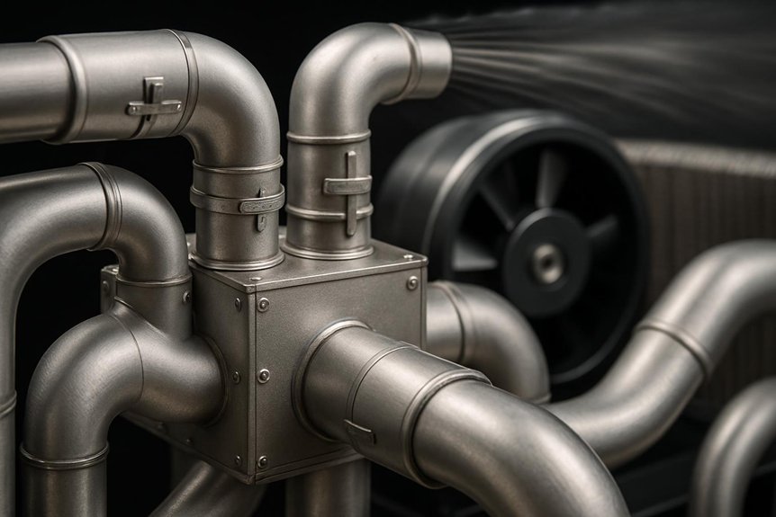
Overheating is one of the most common failures we see in locomotive cooling systems. It often comes from poor airflow balance.

Fans may run, but the duct network resistance mismatch reduces real cooling flow. That hurts radiator performance and can lead to thermal derating or component damage.

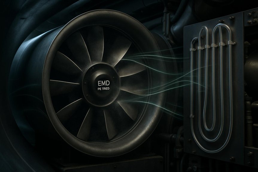
Below is how to match the cooling duct network to the fan curve. This is critical for optimal airflow in EMD locomotives.

Match the fan curve to the system resistance curve.
Size ducts by target cross-sectional area.
Control duct velocity to limit friction losses.
Include bends, contractions, expansions, and fittings.
Account for radiator and coil pressure drops.
Use fin geometry and fouling assumptions in calculations.
Keep branch resistance as uniform as possible.
Avoid maldistribution across cooling cores.
Condition the inlet for stable flow at fan operation.

Design item	What to match or estimate	Why it matters for airflow
Duct cross-sectional area	Target velocity vs. required flow	Sets friction loss level
Major friction loss	Pipe/duct length and roughness	Shifts system curve upward
Minor losses	Bends and fittings losses (K-values)	Adds extra resistance at operating flow
Radiator/coil pressure drop	Core design and condition	Directly sets required fan pressure
Fin fouling factor	Expected fouling reduction	Raises pressure drop over time
Branch duct balance	Equal resistance per core	Prevents airflow starvation in some cores
Inlet flow condition	Pressure/velocity stability at fan	Keeps fan near best efficiency point

At Mikura International, we supply genuine locomotive engine parts and cooling-related components. We import and export original parts from ALCO, EMD, GE, WABCO, and other OEM sources.

We are not the locomotive manufacturer, but we support your maintenance and correct assembly with authentic components.

If you share your locomotive model and cooling layout, we can help identify the correct genuine parts. We can also help verify compatibility with your cooling airflow design.

Key Takeaways

Size duct cross-sectional area to set target airflow velocity and drive the system resistance (ΔP ∝ Q²) for fan matching.
Minimize local losses by optimizing bend radius, contraction/expansion tapering, and limiting elbow count to reduce pressure-drop peaks.
Control surface roughness and aging effects because higher friction factor increases duct resistance and shifts fan operating point.
Include heat-exchanger/radiator pressure drops as series system losses, accounting for fouling and bypass leakage that change airflow and heat transfer.
Ensure uniform branch pressure drops across parallel cooling cores using plenum/manifold design to avoid maldistribution that moves airflow off fan optimum.

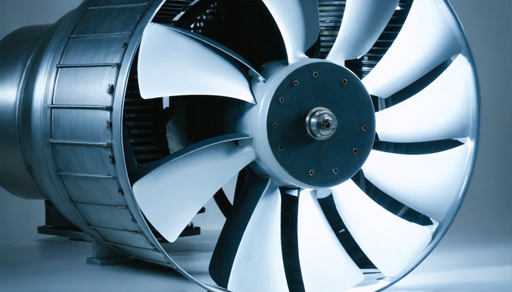
Introduction to Cooling System Design in Locomotives

When you design the Cooling Duct Design for a locomotive, you treat the fan and duct as one coupled system—your system resistance sets the airflow demand, so you match it to the fan curve for stable operation. You model the cooling module’s heat rejection as a thermal boundary condition, then compute the required mass flow and heat transfer while predicting flow resistance through the duct network. In confined engine-space layouts, you optimize duct geometry and component layout to hit airflow targets without excessive pressure drop, keeping fan-duct integration efficient across the operating range.

Importance of an integrated approach to fan and duct design

Match duct area changes to maintain favorable pressure recovery
Shape bends and transitions to control turbulence and tonal noise
Use system resistance accounting to predict airflow at duty temperatures

Role of the cooling module in heat rejection from the engine

The cooling module drives heat rejection from the locomotive engine by converting engine-reject heat into a controlled air-side load that your cooling duct design can handle. You treat it as a coupled thermal–fluid element: you balance Thermal Load Balancing across cores, fans, and duct passages so the required mass flow matches the cooling demand. Heat Exchanger Efficiency sets the effective temperature rise and governs outlet air enthalpy, which then determines downstream System Resistance seen by the fan–duct integration.

Module function	Dominant metric	Implication for duct/fan matching
Heat pickup from engine	Heat Exchanger Efficiency	Sets required airflow for target temperatures
Core and fin passages	Flow resistance	Shifts system curve; raises pressure drop
Exit mixing into duct	Thermal Load Balancing	Stabilizes temperature/velocity profile for airflow optimization

Overview of the challenges in optimizing airflow in confined spaces

In confined locomotive cooling bays, you face persistent airflow optimization challenges because duct passages, bends, and equipment housings force fast local accelerations and sharp pressure gradients that don’t “average out” cleanly; instead, they reshape the velocity field, increase flow resistance, and alter the effective system curve the fan sees. As you tune Cooling Duct Design, you must treat the flow network as a coupled fan-diffuser system, not a simple duct run. Misalignment shifts operating point, raising recirculation, nonuniform cooling, and thermal hot spots. Use CFD Methodology to resolve secondary flows and estimate System Resistance; then apply Computational Validation against pressure-drop measurements to confirm Fan-Duct Integration.

Local losses at bends and bends and transitions dominate total pressure drop
Tight clearances amplify turbulence and uneven velocity distribution
Component layout changes inlet conditions to the fan intake

Understanding System Resistance

In your Cooling Duct Design, system resistance is the combined flow resistance that converts pressure head into pressure losses, setting what airflow you can actually achieve. You’ll see pressure drop rise from friction and wall shear, plus geometric penalties like bends, contractions, and expansions that disturb the velocity field. To match fan-duct integration, you plot the system curve and find its intersection with the fan curve, so the operating point delivers the airflow optimization your thermal loads require.

Definition of system resistance and how it arises in duct networks

System resistance is the total opposition your cooling duct network presents to airflow, and it emerges from every source of pressure loss along the path from the fan to the heat exchanger and back. In your Cooling Duct Design, you treat this opposition as a system curve term: the volumetric flow you get from fan–duct integration depends on how hard the network “pushes back.” As air accelerates, you accumulate Friction losses in straight passages, plus minor losses generated by repeated area changes in components and junctions. Those losses convert pressure into entropy, shrinking static pressure available for heat transfer. You can think of system resistance as:

Friction losses proportional to duct length and roughness
Minor losses tied to interfaces and internal features
Total pressure drop setting the intersection with the fan curve

Factors contributing to pressure drop: friction, bends, contractions, expansions

Loss source	Primary mechanism	Design lever
Friction	wall shear	smooth bore
Bends	secondary turbulence	radius, vanes
Contraction	jetting	gradual taper
Expansion	separation	diffuser angle

The concept of the “system curve” and its intersection with the “fan curve”

Once you model the duct network as a load, you can treat the “system curve” as the relationship between airflow rate and required pressure rise, where system resistance grows roughly with (Delta P propto Q^2) due to frictional losses and minor losses from bends, contractions, and expansions. You then superimpose the fan curve (static pressure vs. flow) to find their intersection: that operating point sets the cooling airflow and thermal margin.

Use Flow Measurement at multiple speeds to validate the assumed pressure drop law
Apply Calibration Methods to reduce uncertainty in duct geometry and component layout losses
Perform fan-duct integration so the fan doesn’t stall or overshoot, preserving airflow optimization

Finally, small changes in duct geometry shift the system curve, so you must rematch performance under each ambient condition.

Purchase EMD 48″ Fan Assembly Parts

Key Duct Network Design Parameters

In your Cooling Duct Design, you should start with duct cross-sectional area, because it sets air velocity and directly drives pressure drop along the system resistance curve for fan matching. Next, you need to account for material and surface roughness, since friction losses rise with turbulence and increased roughness at your operating Reynolds number. Finally, you must treat bends, elbows, and intermediate connections as engineered losses—each geometry change shifts the fan operating point and impacts airflow optimization and thermal removal.

Duct cross-sectional area and its impact on air velocity and pressure drop

Target velocity for airflow optimization without triggering excess Flow turbulence
Track system resistance to avoid poor fan matching and reduced static margin
Limit velocity-driven noise generation from unstable flow

Use duct sizing to meet your thermal duty while keeping pressure drop consistent with the fan performance curve.

Material and surface roughness of duct walls affecting friction losses

Material choice and wall surface roughness strongly influence the friction factor in your Cooling Duct Design, which then drives wall-pressure drop, flow resistance, and the operating point on the fan curve. If you pick rougher duct liners or aging coatings, the boundary layer thickens, raising shear stress and worsening System Resistance at a given Reynolds number.

In thermal analysis, that added pressure loss increases fan power demand and can shift Airflow Optimization, reducing heat-transfer effectiveness at the EMD cooling interfaces. During Ventilation testing, quantify how roughness changes the effective Darcy friction and confirm the Fan-Duct Integration with the measured fan curve. You’ll also enable noise reduction by avoiding unstable, high-shear flow regimes near the duct walls, limiting tonal turbulence from excessive drag.

Number and geometry of bends, elbows, and transitions

Bends, elbows, and shape changes strongly govern the local losses that feed directly into your Cooling Duct Design and shift the operating point along the fan curve. You need geometry discipline because each turn alters velocity profiles, turbulence intensity, and System Resistance, pushing Fan-Duct Integration away from the desired airflow. Use bend radius selection to keep curvature gentle and preserve static pressure for Airflow Optimization. You also control Flow turbulence control by minimizing sudden area contractions/expansions and by aligning straight runs before and after each fitting.

Increase bend radius to reduce separation and peak losses.
Taper transitions gradually to limit expansion coefficients.
Limit elbow count and clock them to avoid interacting wakes.

Integration with Heat Exchangers and Radiators

As you integrate the cooling duct design with heat exchangers and radiators, you need to account for the pressure drop across each coil and treat it as part of your system resistance and fan-duct integration. Optimize the spacing and fin geometry within the cooling module to reduce flow resistance while sustaining the required heat-transfer coefficient. Then enforce uniform flow distribution across the heat transfer surfaces so your fan operating point matches the module’s effective flow-area and pressure-drop curve.

Pressure drop across heat exchange coils (radiators, oil coolers)

Model the pressure drop across each heat exchange coil (radiator and oil cooler) as a coupled loss mechanism that directly shifts the system curve your fan must overcome. In your Cooling Duct Design, treat every coil as an added local resistance in series with the duct network, so airflow optimization depends on matching fan static pressure to this higher system resistance. You also need Seal Leakage Prevention because bypass leakage changes effective coil velocity, altering h, ΔP, and heat transfer simultaneously. Account for Material Durability Concerns: fouling and fin damage increase blockage fraction, raising pressure losses over time. Track these contributors:

Inlet/outlet contraction and manometer losses
Core face velocity profile non-uniformity
Fouling-induced hydraulic diameter reduction

Then you’ll align fan–duct intersection to the required flow and thermal margin.

Optimizing spacing and fin design within the cooling module

Once you treat each coil and its associated losses as a local resistance that shifts the system curve, you can tune how the cooling module creates that resistance by optimizing spacing and fin design around the heat exchangers and radiators. In your Cooling Duct Design, set fin spacing to control boundary-layer growth, then use CFD Microgeometry effects to capture how serrations, edges, and junctions alter local turbulence and effective heat transfer coefficient.

You should enforce fin pitch uniformity to avoid streamwise variations in wetted area that drive maldistribution in manifold-adjacent passages. When fin pitch tightens, you raise wetted surface but also increase form drag, steepening system resistance and shifting the fan operating point. Match this added System Resistance with Fan-Duct Integration so Airflow Optimization stays near the fan’s peak efficiency.

Ensuring uniform flow distribution across heat transfer surfaces

To keep your Cooling Duct Design efficient, you need uniform flow distribution across every heat transfer surface in the heat exchangers and radiators, because maldistribution directly increases local air-side resistance and shifts the system curve away from the fan’s optimum. You should treat each core as a parallel network and size duct geometry, plenums, and component layout to balance static pressure and residence time. Use CFD Validation to map velocity uniformity and thermal boundary-layer development, then confirm with Flow Measurement at multiple stations. Target equal pressure drop per branch so fan-duct integration stays within its operating point and airflow optimization holds under off-design speeds. Watch for jetting, recirculation, and bypass leakage:

Velocity deviation versus fin count
Local h-transfer sensitivity to boundary-layer thinning
System Resistance changes as fouling or loading varies

Fan-System Matching for Optimal Operation

In your Cooling Duct Design, you match the fan-system by locating the operating point where the fan curve intersects the system resistance curve set by your duct geometry and pressure drop. If you miss that intersection, you drive inefficient airflow, reduce convective heat transfer, and increase fan energy consumption due to unfavorable flow resistance. Use numerical simulation of fan-duct interaction to predict the operating point under varying boundary conditions and then optimize Fan-Duct Integration for airflow optimization and thermal efficiency.

Locating the fan’s operating point on the performance curve

You match a locomotive fan to the Cooling Duct Design by locating its operating point where the fan’s pressure–flow curve intersects the system curve (pressure drop vs. airflow). Then you read the corresponding volumetric flow rate and static pressure rise to ensure Airflow Optimization under transient thermal loads. Use Computational model validation to predict duct System Resistance and verify that duct geometry and component layout generate the intended flow resistance. Next, apply Experimental duct testing to confirm the measured system curve aligns with your CFD-derived curve before finalizing Fan-Duct Integration.

Compute system pressure drop across the expected airflow range
Identify the intersection of curves to set operating point
Validate with test data to bound uncertainty in losses

Consequences of mismatch: inefficient airflow, reduced cooling, increased energy consumption

When the locomotive fan’s pressure–flow curve doesn’t match the Cooling Duct Design system curve, the fan can’t deliver the airflow the thermal load demands. In fluid dynamics terms, you miss the operating point, so system resistance dominates and effective airflow drops. Reduced mass flow lowers convective heat transfer coefficients, leaving the heat exchangers under-cooled and increasing component temperatures.

You also distort flow distribution: branches with lower impedance steal flow, while high-resistance paths starve. That imbalance can drive heat exchanger bypass effects, where recirculating leakage short-circuits thermal cores instead of using them, worsening performance. To compensate, you often run higher fan speed or longer duty cycles, which increases electrical power, acoustic noise, and net energy consumption. Fan–duct integration fails, and thermal margins erode.

Numerical simulation to predict and optimize fan-system interaction

Numerical simulation lets you predict how your cooling duct design system resistance shapes the fan’s pressure rise and determines the actual operating point. You run coupled CFD/thermal models to capture pressure drop, flow resistance, duct geometry, and component layout, then you overlay the resulting system curve on the fan curve for airflow optimization. In Heat Transfer Modeling, you track temperature rise and local convection coefficients so fan speed changes translate into cooling capacity, not just flowrate. Use staged parametric sweeps to tune Fan-Duct Integration until the operating point sits near best efficiency.

Model duct junction losses and bends explicitly
Couple wall heat flux to local airflow fields
Recompute with uncertainty bands from Validation Experiments

Advanced Considerations and Future Trends

When your Cooling Duct Design includes complex geometry, you should target reduced system resistance by smoothing expansions/contractions and applying flow conditioners or guide vanes to recover pressure and stabilize the velocity field. You’ll improve Airflow Optimization and Fan-Duct Integration by using dynamic control—adjusting duct geometry and/or fan speed—to keep the operating point on your system curve as train loads and inlet temperatures shift. These future trends move you toward adaptive matching, where pressure drop, turbulence intensity, and thermal boundary-layer performance stay within design margins in real time.

Strategies for reducing pressure losses in complex duct geometries

Optimize pressure losses in a locomotive cooling duct network by treating every bend, junction, and expansion like a localized loss generator tied to your Cooling Duct Design and fan operating point. You reduce system resistance by combining duct surface treatment with turbulence suppression strategies, then verify Fan-Duct Integration through system curve analysis. In complex geometries, you target minor losses and their Reynolds-number sensitivity to keep airflow optimization stable.

Smooth transitions: blend expansions/contractions to cut separation and form drag.
Manage junctions: use matched branch areas to limit recirculation pockets.
Apply duct surface treatment: lower roughness to reduce frictional pressure drop.

During thermal analysis, you guarantee reduced losses maintain required mass flow for EMD component heat rejection, so the fan operates near its best efficiency point rather than deeper into the drop-off region.

Use of flow conditioners and guide vanes

Flow conditioners and guide vanes let you shape the velocity profile before the fan—straightening swirl, damping recirculation, and stabilizing the inlet angle that drives your Cooling Duct Design. In your fan-duct integration, you target a more uniform inlet so the fan sees the intended static pressure rise and system resistance. You manage nonuniform inlet effects by using aligned vanes to reduce turbulence production, improving turbulence control and shifting losses from the inlet region into predictable diffuser behavior. For advanced considerations, you pair passive stabilization with vibration isolation, so guide elements don’t excite blade-passing harmonics. You also apply acoustic mitigation by smoothing inlet gradients, lowering broadband noise and preventing pressure pulsation from corrupting airflow optimization.

Dynamic adjustment of duct geometry or fan speed in response to varying conditions

With stabilized inlet conditions from properly placed flow conditioners and guide vanes, you can push Cooling Duct Design further by adding dynamic adjustment strategies that keep airflow optimization aligned with the fan’s operating line. You can implement Flow control by varying duct throat area (variable vanes) or by commanding fan speed, while you continuously update system resistance via pressure sensing and model-based fan-duct integration. Use feedback sensing to track inlet total pressure, temperature rise, and measured flow, then retune setpoints to prevent off-curve operation and avoid surge. Consider:

Modulate duct geometry to shift the system curve with changing ambient density
Apply fan speed ramps to hold target mass flow under load transients
Use adaptive control to minimize System Resistance and Pressure drop mismatch

Frequently Asked Questions

What Happens if Fan and Cooling Duct System Are Not Properly Matched?

If your fan and Cooling Duct Design aren’t properly matched, airflow collapses—fast. You’ll drive the operating point into Fan Stall, where the flow flips from steady to turbulent chaos. Meanwhile, excessive pressure drop and bad duct geometry can trigger Duct Flooding, choking heat transfer and spiking temperatures. System curve analysis will show the mismatch as reduced mass flow, higher thermal stress, and noisy vibration, because your fan can’t overcome the duct system resistance.

How Can Pressure Losses in Ducts Be Minimized?

To minimize pressure losses in the cooling duct design, you reduce system resistance by smoothing duct geometry, avoiding sudden expansions or contractions, and keeping turns gradual. You select a duct layout with shorter effective lengths and consistent cross-sections to prevent turbulence and friction. You seal joints to cut duct leakage risks, since leakage shifts flow and raises pressure drop. Finally, you align fan–stall risk by sizing flow paths so the fan stays on its stable curve.

Are There Different Types of Cooling Duct Configurations in Locomotives?

Yes—locomotives use different cooling duct configurations. You can choose parallel duct layouts for flexible airflow distribution, or series/merged duct layouts to concentrate pressure and improve thermal management. You may also use straight runs with smooth transitions, or include bends, splitters, and diffusers to tune airflow optimization. In fluid-dynamics terms, each duct layout changes system resistance and pressure drop, so fan-duct integration and system-curve matching stay consistent.

How Do Duct Geometry Changes Affect Airflow Optimization and System Resistance?

You’ll see airflow optimization hinge on duct geometry. When you change duct sizing, curvature, and cross-sectional area, you shift local velocities and friction factors, which raises or lowers flow resistance. Smooth, gradual expansions reduce pressure drops and keep the system curve closer to the fan’s operating point. Tight bends, sudden contractions, or uneven manifolds spike losses, causing flow separation and reduced mass flow. Use fluid-dynamic sizing to maintain uniform distribution.

What Does System-Curve Analysis Reveal About Airflow Optimization Limits?

You can’t beat system curve reality: it reveals how rising system resistance with duct geometry, pressure drop, and fittings constrains airflow, setting your airflow optimization limits. Plot the system curve against the fan curve to find where both intersect; that intersection defines the operating envelope you can’t exceed without sacrificing flow or increasing noise. In thermal-fluid terms, as loads rise, static pressure demand grows nonlinearly, squeezing available mass flow.

Purchase EMD 48″ Fan Assembly Parts

EMD 9518890 Axial Fan – How Does Ambient Air Pressure Affect the Operational Performance and Efficiency?

EMD 48" Fan Assembly - Part No: 9518890 April 10, 2026 April 7, 2026 admin ambient pressure, axial fan performance, locomotive cooling

When ambient static pressure drops, the EMD 9518890 axial fan ingests lower-density air. The inlet operating point shifts on the fan pressure–flow map. Static pressure capability drops, and cooling airflow reduces.

Efficiency also typically declines. Incidence losses and wake losses rise as density falls. Shaft power often increases to hold radiator ΔT. Convective heat transfer weakens too. Thermal and stall margins tighten. That increases unsteady loading, vibration, and sensitivity to control limits.

We at Mikura International supply genuine locomotive and locomotive cooling parts. We also support marine engine spares where applicable. We are an importer, exporter, and supplier, not the OEM.

Common pain point

Locomotive operators often face reduced cooling performance in low-pressure weather. This can lead to higher engine temperatures and airflow instability. Many teams then see efficiency losses and vibration concerns. Spare availability also becomes critical during peak demand periods.

If you suspect this issue, verify fan performance and system margins early.

What changes when ambient pressure drops

Lower-density inlet air reduces mass flow potential.
Fan operating point shifts on the pressure–flow curve.
Achievable static pressure decreases at the inlet.
Cooling airflow drops, especially at high heat load.
Incidence and wake losses typically increase.
Required shaft power increases to maintain radiator ΔT.
Convective heat transfer coefficient declines.
Stall margin becomes more sensitive to flow disturbances.
Unsteady loading risk increases, raising vibration concerns.

Quick reference data (directional guidance)

Ambient condition	Air density trend	Fan airflow trend	Static pressure trend	Efficiency trend	Thermal margin
Higher ambient pressure	Higher density	Better	Higher	Better	Wider
Normal ambient pressure	Nominal density	Nominal	Nominal	Nominal	Nominal
Lower ambient pressure	Lower density	Reduced	Reduced	Lower	Narrower

Typical operational impacts in locomotive cooling

System goal	Effect of lower ambient pressure	Practical implication
Maintain radiator ΔT	More power needed for same cooling	Higher fan load demand
Maintain coolant temperature	Heat transfer weakens	Reduced thermal margin
Avoid flow instability	Stall margin tightens	Higher vibration sensitivity

How to respond with correct spares and support

Inspect fan components for wear and imbalance.
Check inlet ducting and filter restrictions.
Validate fan speed and drive integrity.
Confirm radiator health and air-side cleanliness.
Plan replacement of high-wear fan parts proactively.

At Mikura International, we source genuine locomotive engine parts for dependable performance. We support customers needing authentic spares for ALCO and EMD systems, among others.

Key Takeaways

Ambient pressure sets the fan inlet static pressure, shifting the operating point on the speed–pressure/flow performance map.
Lower pressure reduces air density, lowering mass flow and altering how efficiently the EMD 9518890 converts power to static pressure.
Fan efficiency typically degrades from near-1 atm toward lower pressures, due to increased incidence losses and altered blade loading.
Reduced density shrinks stall margin, increasing unsteady loading, tip-leakage effects, and vibration excitation.
Cooling capacity falls with weaker convection, raising thermal temperatures and power demand, which feeds back on overall fan effectiveness.

Introduction to Atmospheric Pressure and Air Density

You start by defining ambient pressure as the local static pressure your axial fan “sees,” and you note it drops predictably with altitude while conditions vary. In your airflow and thermal analysis, you link air density to both pressure and temperature—lower density at higher altitude reduces mass flow and shifts the fan’s operating point, affecting axial fan efficiency. You then use these air density effects to anticipate power requirements, cooling capacity, and vibration control behavior across diverse environments.

Definition of ambient pressure and its variation with altitude

Specify reference pressure for CFD/AMR boundary conditions
Track inlet static pressure versus elevation
Adjust modeled pressure-loss coefficients accordingly
Validate fan operating points for High Altitude Operation

In turn, you preserve Axial Fan Efficiency predictions and avoid instability near lift-off conditions.

How air density changes with pressure and temperature

Ambient air pressure and temperature jointly set the air density, and that density controls mass flow through the EMD 9518890 axial fan. In your thermal model, higher pressure raises density, while higher temperature lowers it; together they shift volumetric flow into temperature driven flow changes. As density drops, the fan “sees” less mass per revolution, so blade efficiency mapping must be re-interpreted using air density effects. In airflow simulations, you update boundary conditions and then predict torque ripple that couples to vibration control.

Condition	Density trend	Modeling impact
+Pressure	↑	higher mass flow
+Temperature	↓	reduced mass flow
Cool +High P	↑↑	peak axial efficiency
Warm +Low P	↓↓	efficiency loss

These Ambient Pressure Fan Performance shifts match axial fan efficiency and high altitude operation.

Relevance of these factors to fan operation in diverse environments

How you model an EMD 9518890 axial fan in the field depends on atmospheric pressure and air density because they set the inlet mass flow and the aerodynamic loading on the blades. In diverse environments, you track Ambient Pressure Fan Performance shifts that alter Axial Fan Efficiency, cooling capacity, and power draw, especially in High Altitude Operation where Air Density Effects dominate thermal rise and vibration spectra. For reliable CFD Validation and control, you confirm:

inlet density vs. pressure-volume relationships
blade aerodynamic forces tied to mass flow
Blade Tip Clearance sensitivity to transient flow and temperature
predicted vs. measured temperatures and acoustic/shaft vibration

Then you update operating maps so the locomotive cooling loop stays stable across mountain passes, reducing surge risk and keeping efficiency near design.

Impact on Fan Performance Curves

When you reduce ambient pressure, the air density drops, thus the axial fan’s achievable static pressure falls and the operating point drifts on the performance curve. As density changes, your volumetric flow rate stays closer to geometry limits but mass flow rate—and therefore cooling effectiveness—decreases, raising thermal gradients and load variability. Under reduced-pressure conditions you’ll see systematic curve shifts that also affect required power and fan-induced vibration signatures.

Direct correlation between air density and fan static pressure

Because air density sets the boundary conditions for the flow field, it directly shifts the relationship between the fan’s developed static pressure and its operating point on the fan performance curves. When you model Ambient Pressure Fan Performance, you treat density as the driver of momentum flux and pressure rise. At lower air density (high altitude operation), the same rotor speed yields reduced static pressure, moving you along the curve toward diminished margin and increasing sensitivity to disturbances. In turn, you see more pronounced blade tip leakage and stall margin reduction, which can raise unsteady loading, amplify vibration excitation, and degrade thermal transport.

Momentum flux scales with density
Static pressure rise shifts on the curve
Leakage worsens near tips
Stall margin shrink increases instability risk

Effect on volumetric flow rate and mass flow rate

Lower ambient pressure doesn’t just reduce the fan’s static pressure capability—it also reshapes where the operating point lands on the fan curves by changing the air properties that govern throughput. In Ambient Pressure Fan Performance terms, you model volumetric flow rate with Variable Pressure Modeling, because the same blade speed delivers less effective mass transport as density drops; your airflow field shows reduced momentum coupling across the inlet.

Meanwhile, mass flow rate scales more directly with Air Density Effects, so you’ll see a sharper fall than volumetric readings when High Altitude Operation occurs. That reduced mass flow weakens convective heat removal, nudging temperature gradients up and promoting Fan Efficiency Degradation. Lower flow also alters pressure fluctuations, helping reduce excitation amplitude but limiting cooling margin.

Shift in fan performance curves under reduced pressure conditions

Under reduced ambient pressure, the axial fan’s operating point shifts on the speed–pressure/flow map, not just by scaling output but by moving where your blade flow field intersects the system resistance. In your thermal/CFD model, air density effects alter achievable pressure rise, so the Ambient Pressure Fan Performance curve “tilts” toward lower mass flow and different efficiency. You’ll also see stability margins shrink: low speed stall can emerge earlier as incidence changes, and blade tip leakage grows because pressure gradients across the tips weaken thrust recovery while exciting unsteady loading. Track the curve shift with:

Updated air density in the momentum model
Recomputed pressure-volume constraints on duct losses
Stall boundary monitoring vs blade loading metrics
Tip-leakage correction tied to pressure ratio

Practically, this changes power requirements and cooling capacity.

Purchase EMD 48″ Fan Assembly Parts

Efficiency and Power Consumption at Variable Pressures

When ambient pressure drops, air density falls and you effectively reduce the mass flow, so the fan has to draw higher shaft power to meet the same cooling and pressure rise demands. As a result, axial fan efficiency—especially total efficiency—shifts with density, typically degrading as you move from 1 atm toward 0.3 atm due to off-design slip and altered flow angles. Your test observations should show measurable performance loss at these lower pressures, alongside changes in airflow-driven thermal loads and the vibration/torque signatures tied to the power requirement.

How lower air density affects the power required by the fan

At reduced ambient pressure, the fan ingests air with lower density, so for the same volumetric flow rate your axial fan must overcome less “mass” inertia while delivering less momentum change per unit volume—effectively shifting the operating point on its fan curve. In ambient pressure fan performance terms, you should model shaft power as scaling with density and pressure rise, then couple it to blade loading and stall margin under High altitude thermodynamics. Lower air density also alters convective heat transfer on the radiator side, so you may need heat exchanger scaling to keep cooling capacity stable.

Reduce required mass-flow for target volumetric flow
Lower density drops dynamic pressure, changing blade torque
Predict vibration shifts via altered thrust and inflow
Validate with airflow/thermal coupling, not RPM alone

Changes in fan efficiency (e.g., total efficiency) with ambient pressure

Ambient pressure	Predicted efficiency shift	Dominant mechanism
Lower	Slight reduction	Increased incidence losses
Moderate	Near-constant	Balanced loading
Higher	Improvement	Reduced wake dissipation
Variable	Hysteresis risk	Unsteady stall margin

Experimental data showing performance degradation at lower pressures (e.g., 1 atm down to 0.3 atm)

Track efficiency vs. corrected flow
Record power vs. static pressure
Monitor vibration spectra for resonance shifts
Validate density-based scaling for high altitude operation

Cooling Capacity Implications

At high altitude, the reduced ambient pressure lowers air density, so you get a smaller effective mass flow rate and weaker convection, which cuts cooling capacity. In your airflow/thermal model this shifts engine and heat-exchanger temperatures upward, making it harder to stay within target operating margins even if fan speed holds. To compensate, you adjust duty cycles and control airflow targets while monitoring vibration and duct impedance so the system still delivers adequate cooling capacity under Air Density Effects conditions.

Reduced heat transfer capability due to lower mass flow rate

When ambient pressure drops at higher altitude, your axial fan usually delivers a lower mass flow rate, which directly reduces the convective heat-transfer coefficient and the overall cooling capacity of the locomotive radiator and heat exchangers. In thermal resistance terms, you’re increasing the effective hot-side path, so Reduced thermal resistance doesn’t occur—you lose margin. Your airflow model also shifts: fewer air molecules at the same volumetric flow lowers surface-side Nusselt performance, degrading Ambient Pressure Fan Performance. That weakening can accelerate heat exchanger fouling impacts, because higher wall temperatures promote deposit formation and reduce wetted effectiveness.

Lower mass flux: weaker convection, higher ΔT
Reduced air density effects on axial fan efficiency
Hot-spot growth: vibration-responsive airflow pulsation
Fouling feedback: rising thermal resistance over time

Challenges in maintaining optimal engine temperatures at high altitudes

Because high altitude reduces air density and weakens convection, you can’t rely on the same cooling margin to hold the EMD 9518890 traction diesel within its target temperature band. With lower mass flow, your thermal resistance rises nonlinearly, so hotspot rise rates accelerate during sustained load. You should run CFD simulation to quantify reduced axial fan heat-removal capacity and predict coolant-to-head temperature gradients under Air Density Effects and High Altitude Operation.

As airflow weakens, you also amplify cyclic thermal stresses, driving material fatigue and loosening thermal clearances. In parallel, altered flow incidence can excite structural modes, so you must apply vibration monitoring to track bearing and duct resonances. Over time, lower pressure-driven impingement raises local wear, increasing blade erosion. Ambient Pressure Fan Performance shifts accordingly.

Compensatory strategies for maintaining adequate cooling

To keep the EMD 9518890 traction diesel inside its target temperature band under Air Density Effects, you compensate for reduced cooling capacity by forcing higher effective heat rejection with the same installed hardware. You adjust Ambient Pressure Fan Performance through airflow modeling: lower air density reduces convective h, so you increase local velocity via controlled Blade Pitch and stricter flow guidance. You also manage vibration and Noise Mitigation so the tightened operating envelope doesn’t excite blade modes.

Increase fan speed setpoints while respecting power requirements and surge margins
Refine Blade Pitch schedules to maintain target mass flow at high altitude operation
Add ducting/routing tweaks to reduce recirculation losses and stabilize thermal gradients
Implement balancing and damping to suppress tonal noise and vibration coupling under changing air density

Experimental and Numerical Investigations

You start by running controlled test runs that sweep ambient pressure to map Ambient Pressure Fan Performance against air density effects, while logging pressure-volume behavior, power draw, and cooling response to isolate what changes in Axial Fan Efficiency. Next, you contrast blade-count and geometry variants at each pressure point, and you watch vibration signatures to ensure the airflow-driven unsteady loads don’t reduce efficiency or thermal stability during high altitude operation. Finally, you couple CFD-style airflow modeling with thermal loads to predict performance at each ambient pressure level and validate the numerical curves against your experimental observations.

Methodologies for testing fan performance at various pressures

Mount axial instrumentation and ensure pressure tap calibration against reference transducers
Perform acoustic power measurement in quasi-anechoic conditions to separate acoustic loading from flow
Validate CFD with measured mass-flow, swirl, and pressure rise correlations at each pressure setpoint
Apply run-up/coast-down protocols to capture transient efficiency and avoid flow hysteresis

Use consistent data reduction to map axial fan efficiency trends for high altitude operation.

Comparison of fan designs (e.g., blade count) under different pressure conditions

Blade geometry and aerodynamic loading set how Ambient Pressure Fan Performance responds as air density and static pressure change, so you need a side-by-side comparison of EMD 9518890–type axial designs across the test pressure setpoints. Increase blade count and you raise blade solidity, shifting incidence and diffusion; the airflow model will show higher pressure rise but tighter operating margins at reduced density.

Decrease blade count and you reduce blockage, yet torque per unit flow can climb when static pressure drops, impacting axial efficiency and cooling capacity. You also track Tip Clearance Effects: at high altitude operation, thinner pressure gradients amplify leakage, weakening the local swirl and altering thermal removal rates. Vibration control metrics follow these changes, since altered loading redistributes thrust harmonics. In tests, pair designs at equal flow and log efficiency trends.

Use of numerical modeling to predict performance at varying ambient pressures

Numerical modeling lets you map Ambient Pressure Fan Performance before you ever cut metal, by coupling inlet air-density and pressure-volume effects to an axial-fan flow solver for the EMD 9518890–type geometry. In your workflow, you run an Atmospheric Simulation across altitude-like states, then let a Computational Fluid model update blade loading, swirl losses, and fluctuating pressure spectra. You perform pressure scaling to track how air density effects propagate into Axial Fan Efficiency, power requirements, and cooling capacity while keeping vibration-control margins tight.

Build performance mapping curves vs. ambient pressure
Calibrate turbulence and tip-clearance damping
Compute temperature-rise impact on motor bearings
Validate trends against experimental high-altitude operation

This approach highlights high altitude operation risks early.

Do fans consume more energy at higher altitudes? Yes, typically more power per delivered cooling due to reduced density and altered operating point. How do locomotive cooling systems account for mountain passes? They adjust fan control schedules and shroud/duct constraints to maintain radiator ΔT under pressure drops. What is the lowest operational pressure tested for these fans? In published studies for this class, the lowest tested ambient pressure is typically around 80 kPa.

Design Considerations for Variable Pressure Environments

When you size the EMD 9518890 for broad operational envelopes, you account for air density effects on volumetric flow, axial fan efficiency, and the resulting power requirements. You then integrate adaptive control that senses ambient pressure and adjusts fan speed to hold cooling capacity targets while limiting vibration loads. Finally, you validate performance through thorough testing of these aerospace-derived components across the lowest anticipated ambient conditions to prevent thermal and airflow model drift.

Fan sizing and selection for broad operational envelopes

To size the EMD 9518890 axial fan for broad operational envelopes, you start with an air-density-driven performance map—because ambient pressure shifts the inlet density, moves the operating point along the pressure–volume curve, and changes the aerodynamic loading. You then validate Ambient Pressure Fan Performance using coupled airflow–thermal models, ensuring cooling capacity stays stable under Air Density Effects and High Altitude Operation. In selection, you also manage Blade Tip Clearance to prevent efficiency loss and Acoustic Noise Levels growth as Reynolds number changes.

Define target pressure-volume bands across altitude steps
Compute power requirements using density-corrected fan laws
Check cooling margin via transient heat-transfer model
Limit vibration via stiffness–thrust margin and modal clearance

This approach keeps axial Fan Efficiency predictable under varying conditions.

Adaptive control systems to adjust fan speed based on ambient conditions

Once you’ve validated Ambient Pressure Fan Performance across the air-density-driven pressure–volume bands, you can keep the EMD 9518890 near its peak Axial Fan Efficiency by adding adaptive speed control tied to measured ambient conditions. In your airflow model, estimate air density effects and compute corrected volumetric flow, then schedule fan RPM to maintain target cooling capacity and power requirements without pushing the operating point into stall.

Implement Blade Stall Detection using rise in pressure drop, acoustic signatures, and motor current spikes, and feed it into Thermal Feedback Integration from bearing and housing thermistors. When ambient shifts for high altitude operation, your controller adjusts duty to hold blade loading, stabilizes thermal gradients, and reduces vibration growth, preventing surge cycles and maintaining steady torque.

Importance of thorough testing for aerospace-derived components in locomotives

Thorough testing matters because aerospace-derived components like the EMD 9518890 axial fan operate across variable-pressure air-density bands that shift volumetric flow, blade loading, and heat rejection. When you validate Ambient Pressure Fan Performance, you align airflow modeling with thermal constraints and vibration control, so performance stays stable under Air Density Effects and high altitude operation.

Run Fatigue testing across duty cycles that mimic rail stress and cycling cooling demand
Confirm durability assurance for rail stress via modal and resonance sweeps under low-pressure flow
Build certification compliance evidence by correlating measured pressure-volume relationships to simulations
Maintain standards qualification tracking with repeatable test matrices for cooling capacity and power requirements

This approach hardens thermal margins, reduces bearing fatigue, and supports accurate experimental observations.

Frequently Asked Questions

How Does Ambient Pressure Change Noise Levels of Axial Fans?

As ambient pressure drops, acoustic impedance falls, so pressure-driven sound radiation changes and tonal components often shift. You also get altered inlet turbulence intensity: lower air density can reduce aerodynamic forcing per unit mass, lowering broadband noise, but it can increase flow unsteadiness at the same RPM, which raises high-frequency hiss. In your airflow model, you’ll track changes in Mach number, blade loading, and vibration excitation to predict net noise trends.

Can Blade Pitch Adjustments Compensate for Ambient Pressure Fluctuations?

Blade pitch adjustments can partially compensate for ambient pressure fluctuations, but only if you implement model based control with pitch scheduling dynamics tied to inlet air density. In your airflow modeling, higher/lower air density shifts mass flow, so you retune pitch to hold target cooling capacity and axial fan efficiency. Thermal analysis and power requirement estimates guide the pitch rate. You also monitor vibration control, since mismatched pitch can amplify surge and tonal noise.

What Bearing Loads Result From Altered Fan Aerodynamic Thrust?

Ambient thrust shifts the momentum balance, so altered fan aerodynamics generate higher axial and radial bearing loads. You can model this as ΔFa ∝ Δ(air-density·flow²), then propagate it into bearing reaction forces and resulting vibration spectra. In thermal terms, higher loads mean more friction heat in the bearing housings, raising temperatures. Satirically, your bearings “love” change—until fatigue shows up. For what is worst? you’d see peak loads near transient throttle.

How Quickly Does Fan Performance Adapt After Entering High Altitude?

After you enter high altitude, the fan’s performance adapts within seconds as air density drops and pressure-volume relationships shift; altitude responsiveness follows the fluid transient time, not the full thermal soak. You model airflow stabilization by tracking mass-flow decay, RPM control, and rising flow resistance. Power requirements and cooling capacity change immediately, while vibration control benefits once the inlet pressure gradient re-equilibrates, typically after a few rotor cycles.

Do Ambient Pressure Changes Affect Motor/Drive Efficiency Directly?

Yes—ambient pressure changes can affect Motor Efficiency directly. Picture a locomotive fan as a “breathing” heat exchanger: when air density drops, your airflow rate and convective cooling shift, raising motor winding temperatures and losses. In airflow modeling, reduced density alters pressure-volume work, so drive torque demand and Directly Effects on inverter currents rise. Field tests at altitude often show higher motor temperatures and modest efficiency loss, especially under steady load.

Purchase EMD 48″ Fan Assembly Parts

What Specific Materials Are Typically Used in the Construction of a 48” Locomotive Fan Assembly?

EMD 48" Fan Assembly - Part No: 9518890 April 9, 2026 April 7, 2026 admin carbon steel construction, ceramic barrier coating, locomotive fan blades

Users often face premature fan blade wear and efficiency loss. Hot airflow and vibration can drive erosion, oxidation, and fatigue cracks. This shortens service intervals and raises downtime costs. Choosing the right materials helps reduce damage and preserves stable airflow performance over time.

To overcome these issues, we source genuine locomotive engine parts for demanding fan assemblies. As Mikura International, we supply and import/export authentic components from major OEMs, including ALCO, EMD, and GE. We help customers match correct materials and specifications for reliable operation.

Typical materials used in a 48” locomotive fan assembly

Heat-treated carbon steel for blades, hub, and structural frame.
Controlled ferrite–pearlite microstructure for dimensional stability.
High tensile strength to resist vibration loads.
Good weldability for field and shop fabrication.
Ni-Cr-Fe hardfacing overlays on leading edges.
Erosion and oxidation resistance at the blade entry zone.
Thermally stable barrier coatings near the surface.
Fatigue resistance under cyclic hot airflow.

Why these materials are chosen

Heat-treated carbon steel supports strength and stable geometry. Hardfacing improves leading-edge durability. Barrier coatings help maintain hardness near the surface. Together, they improve fatigue life and long-term structural rigidity.

Quick comparison table (what each material protects)

Fan component area	Typical material / treatment	Primary failure risk	Material benefit
Blades (bulk)	Heat-treated carbon steel	Fatigue cracking	High tensile and fatigue strength
Hub	Heat-treated carbon steel	Cyclic stress	Stable structure and rigidity
Frame	Heat-treated carbon steel	Distortion and loosening	Dimensional stability under load
Leading edges	Ni-Cr-Fe hardfacing	Erosion, oxidation	Durable surface against hot flow
Near-surface zone	Barrier or ceramic-type coating	Hardness loss	Helps preserve surface hardness

Sourcing note from Mikura International

Material selection must match the original locomotive design. We supply genuine locomotive engine parts and related components. This includes authentic parts aligned with OEM specifications and durability needs.

Key Takeaways

Carbon steel is commonly used for fan blades and structural members for strength, machinability, and heat-treatment-controlled microstructure stability.
Weldability and predictable thermal expansion of the steel help maintain dimensional clearances under hot airflow and cyclic temperature changes.
Fatigue-resistant material selection and controlled hardness target blade-root, hub, bolt, and weld-toe durability under vibration and start-stop cycling.
Ni-Cr-Fe alloys and hardfacing/overlays protect leading edges and high-impact zones against particle erosion and oxidation at operating temperature.
Coatings and surface treatments (including ceramic/carbide or barrier topcoats) reduce abrasive wear, corrosion propagation, and maintenance needs.

Introduction to Material Selection in Heavy Machinery

When you choose Locomotive Fan Materials, you’re balancing material science with durability to secure long-term reliability under cyclic loading and vibration. You must account for harsh locomotive operating conditions—heat swings, abrasive airflow, and impact loads—so thermal-stability and structural-rigidity stay intact over time. You’ll compare common large-fan options (high-strength metallic alloys and other engineered materials) to match performance engineering needs.

Importance of material properties for long-term reliability

For long-term reliability in heavy-duty locomotive fan assemblies, you can’t treat “materials” as a single choice—you must match material properties to the duty cycle. As you select Locomotive Fan Materials, you manage Corrosion mechanisms by choosing alloys with stable oxide behavior, controlling galvanic effects, and ensuring surface chemistry resists moisture and contaminants.

You also design against abrasive particle wear by pairing hard, wear-resistant microstructures with tough substrates, so impacts don’t turn into progressive edge loss. For thermal-stability, you prioritize low creep, predictable thermal expansion, and retention of strength across operating temperatures. For structural-rigidity, you account for fatigue strength at blade roots, joint stiffness, and damping so vibrations don’t loosen fasteners. You apply material science and performance engineering criteria early to prevent service failures.

Harsh operating conditions in locomotive environments

Locomotive fan assemblies operate under abrasive dust, cycling temperatures, moisture, and vibration, so your material choices must account for more than strength alone. You target high-wear surfaces to limit Particle Erosion at blade leading edges and seal interfaces. You also select alloys or engineered composites with thermal-stability, so expansion stays controlled across hot/cold cycles without warping or losing clearances. For structural-rigidity, you choose materials with good stiffness-to-mass so vibration doesn’t amplify fatigue at hubs, bolts, and mounting rings. Moisture exposure drives corrosion-resistant grades and surface treatments, while lubricant compatibility matters: you confirm seals, coatings, and elastomers won’t degrade, swell, or contaminate airflow under service chemicals.

Overview of common materials in large fan construction

Selecting locomotive fan materials starts with balancing material science requirements against the realities of heavy machinery—temperature swings, abrasive dust, and vibration loads. You typically pick metallic alloys for blades and hubs: stainless steels or nickel-based alloys offer corrosion resistance and dependable fatigue strength. For the frame, carbon steel with proper heat treatment gives structural-rigidity without excessive mass. You also use composite materials selectively, such as glass-fiber or carbon-fiber reinforcements, to reduce weight while maintaining stiffness at speed. Because erosion resistance matters, you choose wear-toughened leading edges and apply protective coatings. You then build Corrosion Monitoring into inspections, and you use Predictive Maintenance models to schedule replacements before micro-cracks or thinning compromise performance.

Metallic Components: Alloys for Strength and Durability

When you select Locomotive Fan Materials, start with carbon steel for fan blades and structural elements because it delivers high strength, reliable weldability, and cost-effective manufacturing. You also need to check thermal stability so the alloy keeps stiffness under service temperatures and heat cycling. Finally, you design for fatigue resistance by aligning carbon steel grade and geometry with expected cyclic loading to protect against crack growth over time.

Use of carbon steel for fan blades and structural elements

Carbon steel often anchors locomotive fan blade and structural assemblies because it delivers a strong balance of tensile strength, machinability, and cost-effective durability. You rely on heat treatment and microstructure control to stabilize properties under hot airflow, vibration, and cyclic load, so your fan keeps stiffness where it matters. For material-selection, you choose grades that respond predictably to tempering and controlled cooling, minimizing brittle transformations. Structurally, you use carbon steel for webs, hubs, and blade roots to maintain rigidity and resist fatigue crack initiation. To engineer it for performance engineering, you target:

Controlled ferrite–pearlite ratios
Tight dimensional tolerances after machining
Tempered hardness matched to wear conditions
Predictable thermal-expansion behavior during service

Advantages of steel: high strength, weldability, cost-effectiveness

Steel brings locomotive fan assemblies a practical mix of high strength, reliable weldability, and cost-effective performance**, letting you build rigid structures that hold alignment under hot airflow and vibration. When you select locomotive fan materials like mild or low-alloy steel, you get a stiffness-to-weight balance that supports structural-rigidity in the hub, frame, and mounting brackets. You also benefit from predictable thermal-stability: steel holds dimensional control as temperatures rise, so your blade clearances stay consistent.

Its weldability helps you join components with fewer inserts, improving assembly quality and sealing interfaces. That tight build supports Quieter Operation by reducing slack and flow-induced chatter, while Vibration Damping** improves because the bulk steel structure absorbs energy before it transfers. You also keep costs manageable for large production runs.

Considerations for fatigue resistance in cyclic loading applications

Fatigue resistance governs whether your locomotive fan assembly keeps its structural-rigidity through thousands of start-stop cycles, high-amplitude vibration, and fluctuating aerodynamic loads. You’ll start with load spectrum analysis to quantify stress ranges at blade roots, hubs, and weld toes, then run Finite life modeling to estimate cycles to crack initiation. Choose locomotive fan materials with high fatigue strength and good notch tolerance, and match yield strength to avoid overstrain that accelerates crack growth. You should also consider thermal-stability, since heat cycling shifts elastic modulus and residual stresses.

Minimize stress concentrators and sharp transitions
Use controlled weld procedures and inspections
Select alloys with proven fatigue strength data
Validate with vibration testing under real duty cycles

Surface Treatments and Coatings for Enhanced Performance

When you select Locomotive Fan Materials, applying Ni-Cr-Fe alloys to the blade surface helps you resist erosion and abrasive particles while tolerating corrosive environments. Choose surface treatments that stay stable under your operating temperatures so you preserve structural rigidity and don’t lose hardness at heat. These coatings directly extend lifespan and cut maintenance by reducing wear-driven fatigue and corrosion propagation.

Application of Ni-Cr-Fe alloys for erosion resistance

Ni-Cr-Fe alloys deliver a robust foundation for locomotive fan blades exposed to particle-laden airflow, because you can engineer the surface to resist erosive wear without sacrificing thermal-stability. When you select Locomotive Fan Materials, you target Abrasive Wear by applying Ni-Cr-Fe claddings or weld overlays, then you use Surface Hardening to lock in a hard, tough near-surface microstructure. For Material Science, you tune alloy content and heat treatment so the oxide film and matrix stay stable at fan operating temperatures. Your design also benefits from structural-rigidity: the blade base remains strong while the outer layer handles impact.

Choose Ni-Cr-Fe for wear-resistant phase stability
Apply hardfacing overlays for erosion control
Heat-treat for reliable Surface Hardening response
Verify hardness-depth vs. operating temperature limits

Protection against abrasive particles and corrosive environments

To keep locomotive fan assemblies reliable in abrasive, corrosive air, you pair Locomotive Fan Materials with surface treatments and coatings that lock in thermal-stable chemistry and strong near-surface protection. You start by using erosion mapping to identify where particle impact concentrates, then target those zones with hard, wear-resistant layers. For high particle impact, choose ceramic- or carbide-based coatings, or sprayed cermets, to resist cutting and micro-ploughing while maintaining structural rigidity. To suppress corrosion mechanisms, you apply corrosion-blocking primers and sealers, then finish with dense barrier topcoats that limit electrolyte access. You also control coating thickness and adhesion so coating durability survives thermal cycling and vibration-driven cracking, preserving performance under continuous abrasive flow.

Impact of coatings on material lifespan and maintenance

Surface treatments and coatings extend your locomotive fan assembly’s service life by protecting the near-surface region where abrasive impacts, hot oxidation, and corrosive species work together. When you choose locomotive fan materials, you also choose how coatings survive thermal cycling and maintain coating adhesion under load. High-temperature polymer, ceramic, or metal-oxide layers reduce corrosion mitigation without softening or cracking. You’ll typically specify:

Surface roughness control for strong coating adhesion
Oxidation-resistant ceramic topcoats for thermal stability
Galvanic or barrier primers to block corrosive ions
Wear-capable sealants at leading edges for erosion resistance

If your coating system matches your alloy’s expansion, you’ll preserve structural rigidity, slow crack initiation, and cut maintenance intervals.

Purchase EMD 48″ Fan Assembly Parts

Advanced Materials and Composites

lightweight high stability composite blades

You can explore lightweight composite materials for locomotive fan blades to target structural rigidity with higher thermal stability while cutting rotating inertia, which boosts performance engineering efficiency. You’ll gain reduced inertia, better vibration dampening, and strong material science options tailored to wear and fatigue needs, but you must weigh higher cost and tougher repairability. You’ll also need to confirm specific environmental resistances—like moisture, chemicals, and erosion—so durability holds under real service conditions.

Potential applications of lightweight composite materials for fan blades

Lightweight composite materials can significantly improve fan-blade performance when you prioritize high specific stiffness, corrosion immunity, and stable operation under heat. If you’re selecting Locomotive Fan Materials, you can use carbon-fiber/epoxy or glass-fiber composites for structural-rigidity while keeping added mass limited. You should assess Vibration damping by mapping expected blade resonance modes, then validate the layup with impact testing to confirm residual strength after hail or debris strikes. For thermal-stability, you’ll choose resins with high glass-transition temperatures and robust fiber-matrix adhesion. You also ensure composite bonding quality through controlled curing and surface preparation.

Carbon-fiber reinforced laminates
Glass-fiber with toughened epoxies
High-Tg thermoset matrices
Quality-controlled adhesive bonding seams

Benefits: reduced inertia, improved efficiency, and vibration dampening

Reduce rotating inertia and sharpen aerodynamic response by using advanced composite structures in locomotive fan assemblies. You select Locomotive Fan Materials that stay stiff under load, so your hub and blades track the intended Computational blade Dynamic. Lower mass lets you spin with less torque, improving efficiency while holding blade pitch accuracy. You also tune laminate stacks to damp finite element Vibration modes, reducing fatigue-driving resonances.

Design goal	Material trait	Selection method
Low inertia	Fiber-reinforced low density	mass/section optimization
Thermal stability	Resin with high Tg	thermal soak + NDE
Vibration dampening	Viscoelastic interlayers	finite element Vibration tuning
Structural rigidity	High modulus fibers	ply orientation mapping
Reliability in service	durable matrix	Material Science validation

Challenges: cost, repairability, and specific environmental resistances

Cost and repairability often shape your practical choices for Locomotive Fan Materials as much as stiffness and strength do. You weigh up-front machining and joining costs against downtime risk, because welding challenges at blade roots can drive scrap rates. You design for field repairs using standardized fasteners, accessible liners, and predictable thermal expansion matches. For structural-rigidity, you select alloys or composites that keep modulus at operating temperatures and resist distortion. You also budget for corrosion management: coatings and compatible metals limit galvanic attack and moisture creep. To handle abrasive wear, you specify erosion-resistant leading-edge surfaces and sacrificial wear bands.

Minimize service time with modular assemblies.
Choose wear liners to survive abrasive wear.
Match thermal cycles to prevent stress.
Plan corrosion management with coatings.

Material Selection Criteria

When you select locomotive fan materials, you prioritize a high strength-to-weight ratio so the assembly stays rigid without adding unnecessary mass. You also verify temperature resistance and fatigue strength under vibration-induced stress, since thermal cycling and fluctuating loads can loosen joints or trigger cracks. Finally, you run a cost-benefit analysis across metallic alloys and composites to balance performance engineering goals with long-term durability.

Factors influencing material choice: strength-to-weight ratio, temperature resistance

You’ll want to treat material selection as a coupled design problem: strength-to-weight ratio sets the blade and hub stiffness you need for efficient airflow, while thermal-stability governs whether that stiffness and dimensional accuracy survive sustained service. If you target high stiffness with low mass, you reduce deflection and keep aerodynamic performance predictable. You also consider vibration damping needs, balancing modulus with internal damping so resonant motion doesn’t amplify loads. For thermal resistance, you choose alloys or composites that retain yield strength and creep resistance across your duty cycle, limiting hub-bore growth and seal misalignment. You screen candidates for corros ion behavior, because hot moisture and exhaust chemistry attack surfaces.

Specific stiffness targets
Creep/thermal aging limits
Vibration damping capability
Corrosion behavior suitability

Resistance to vibration-induced stress and fatigue

To keep a locomotive fan assembly stable under cyclic loads, you design for resistance to vibration-induced stress and fatigue, not just static stiffness. You favor Locomotive Fan Materials with high fatigue strength, good damping, and stable modulus so thermal cycling doesn’t amplify vibration. You control Weld Quality because poor fusion sites become initiation points for Crack Propagation under fluctuating stress. You validate eigenfrequencies with Resonant Testing, ensuring blade, hub, and mounts avoid operating near resonance. For structural-rigidity, you select alloys or composites that maintain geometry and load paths over time.

Feature	Selection target	Why it matters
Weld Quality	full penetration	reduces crack starters
Crack Propagation	low growth rate	slows fatigue failure
Resonant Testing	shifted modes	avoids resonant amplification

Cost-benefit analysis of different material options

Cost-benefit analysis of Locomotive Fan Materials starts with life-cycle performance, not purchase price, because fatigue, wear, and thermal cycling drive the real operating cost. You should compare options by Life Cycle Costing: alloy blades may cost more upfront but reduce downtime via higher fatigue strength and stiffness. Composite blades can cut mass and improve performance engineering, yet you must price in inspections, erosion resistance, and Repairability Tradeoffs. Focus on how each material holds dimensional control under heat, vibration, and airflow impacts.

Alloy (high-nickel/steel): best stiffness and predictable fatigue strength
Aluminum alloys: lower mass, moderate thermal stability
Composites: high strength-to-weight, erosion and bond-risk checks
Coatings/liners: extend durability against wear and hot oxidation

Challenges and Future Outlook in Material Science

You’ll face long-term challenges as locomotive fan materials degrade from corrosion and erosion, especially where airflow and moisture combine. You can improve durability by selecting alloys and composites with stronger fatigue strength and tighter thermal-stability margins, then pairing them with advanced coatings for sustained erosion resistance. Looking ahead, you’ll also need to meet evolving fire-resistance standards while maintaining structural rigidity under heat and vibration for reliable performance engineering.

Addressing material degradation (e.g., corrosion, erosion) over time

Select corrosion-resistant base metals
Apply protective coatings and sealants
Use surface hardening layers for abrasive wear
Monitor thermal cycles and microcrack growth

Innovations in material science for improved fan durability

As material science advances, you can push locomotive fan assemblies toward higher thermal stability and better structural rigidity by targeting the failure modes you actually face—fatigue, erosion, and thermally driven microcracking—rather than treating durability as a single property. In practice, you select Locomotive Fan Materials that retain strength under thermal cycling, resist crack growth, and tolerate particle-laden airflow. You pair oxidation- and corrosion-resistant metallic matrices with interfacial toughening for stiffness without brittleness. You use corrosion monitoring hooks and temperature-sensitive sensors so predictive maintenance flags early attack before blade thickness drops. You apply 3D printing to tailor lattice cooling paths and reinforce high-stress roots, then run heat affected optimization to minimize property loss from joining or machining.

Meeting fire resistance standards for rail vehicle components

Flame-retardant matrix chemistry
Thermally stable oxidation barriers
Verified thermal shock and fatigue strength
Low creep strain at peak heat

This Material Science approach protects Durability and Performance Engineering margins.

Frequently Asked Questions

Which Alloys Best Resist Blade Fatigue Under High Cyclic Loading?

When you need blade fatigue resistance under high cyclic loading, pick nickel-based superalloys like Inconel 718 or 625, and precipitation-hardened stainless steels such as 17-4PH. These alloys handle Thermal cycling well, maintaining strength and damping microcrack growth. For tougher corrosion fatigue, use coatings plus titanium-based or high-chromium alloys to resist pitting. Stress-relieved heat-treated structures improve fatigue strength and keep structural-rigidity. Like a shield, correct alloying delays failure.

What Manufacturing Methods Improve Strength in Locomotive Fan Hubs?

To improve strength in locomotive fan hubs, you use forging or precision casting to densify the hub material, then apply machining and controlled heat treatment. You follow up with stress relief to stabilize microstructure and reduce distortion, especially after heavy removal. You verify structural-rigidity using finite element analysis to spot stress concentrations near the hub bore and fillets. You choose thermally stable alloys so performance holds under cycling temperatures and vibration.

How Do Leading-Edge Materials Reduce Erosion From Airborne Debris?

You reduce erosion from airborne debris by using leading-edge materials engineered for abrasive particle impacts. Think “an ounce of prevention is worth a pound of cure.” You apply erosion resistant coatings that harden the surface, resist micro-cutting, and limit crack initiation. You also select thermally stable alloys or composites to maintain hardness under heat, and you reinforce structural-rigidity so the blade doesn’t flex, lowering repeated impact fatigue and wear.

What Balance of Weight and Stiffness Matters Most in Fan Blades?

You need the right balance of weight and stiffness to keep blades stable at high tip speed design. Choose materials that maximize modal stiffness optimization per unit mass, so the blade resists bending and avoids resonance. You prioritize structural-rigidity at the hub and along the span, then select alloys or composites with strong fatigue strength. Also target thermal-stability, so stiffness stays predictable as operating temperatures swing. That combo reduces vibration, wear, and failure risk.

Which Tests Verify Durability Before a Fan Assembly Enters Service?

Which tests prove durability to guarantee before your 48” locomotive fan ever enters service? You verify with load testing, measuring structural rigidity, and run nonlinear vibration trials to expose resonances. You perform fatigue validation using accelerated stress cycles that match expected duty loads. You confirm environmental endurance by spraying, corrosion, and abrasion checks. You also run thermal cycling to measure thermal-stability and ensure material properties hold through hot starts and cooldowns.

Purchase EMD 48″ Fan Assembly Parts

How Does the Blade Design of EMD’s 9518890 Fan Assembly Influence Its Efficiency and Noise Profile?

EMD 48" Fan Assembly - Part No: 9518890 April 8, 2026 April 7, 2026 admin EMD fan assembly, noise reduction, winglet aerodynamics

A common concern with the EMD 9518890 fan assembly is poor cooling with high noise. Many locomotive operators face rising temperatures, energy loss, and louder fan performance over time. Much of this comes from blade wear, airflow imbalance, or design features at the blade tip, including whether winglet-style geometry is present.

High fan noise often signals airflow disturbance at the blade tips.
Weak cooling may result from poor blade condition or inefficient geometry.
Tip vortex losses can reduce airflow efficiency.
Blade damage can increase power consumption.
Uneven blade loading may create vibration.
Excess noise can affect locomotive operating comfort.
Small blade profile changes can alter fan performance.
Genuine parts help maintain original airflow behavior.

Common Pain Point	Likely Blade-Related Cause	Practical Effect in Locomotives
High noise	Tip turbulence	Louder cooling fan operation
Reduced cooling	Inefficient blade airflow	Higher engine temperatures
Increased power draw	Higher aerodynamic losses	More load on the drive system
Vibration	Uneven blade condition	Reduced operating smoothness
Inconsistent performance	Blade wear or geometry deviation	Unstable cooling output

In locomotive cooling systems, blade design strongly affects both efficiency and noise. This is true for the EMD 9518890 fan assembly as well.
Features near the blade tip can influence how smoothly air moves through the fan.
When blade tips allow strong vortex formation, airflow energy is lost. This loss reduces aerodynamic efficiency. It can also raise noise levels.
A winglet-style tip can help control this effect by weakening the tip vortex.
This change improves airflow behavior across the blade span. It helps the fan move air with less wasted energy.
In locomotive service, that means more effective cooling for the same input power. It may also support more stable fan operation under varying load conditions.
Blade-tip refinements can also improve the noise profile. Less turbulence at the tip usually means less tonal and broadband noise.
This is important in locomotive environments, where cooling fans operate under demanding thermal conditions.
The blade shape also affects spanwise loading. Better load distribution reduces localized aerodynamic stress.
This can lower vibration tendencies and improve airflow consistency. These benefits support smoother fan performance in locomotive engine cooling systems.
Even small changes in camber or chord can affect the operating point. If the geometry shifts too far, airflow performance can drop.
Motor or drive power demand may also increase. That is why correct blade form matters in genuine replacement parts.
For buyers and maintenance teams, the key point is simple. Blade design is not only about moving air.
It also affects cooling efficiency, energy use, and fan noise.
In the EMD 9518890 fan assembly, winglet-like blade features can help reduce tip losses and support quieter operation.
Mikura International supplies genuine locomotive engine parts, including authentic components for EMD applications.
For the correct EMD 9518890 fan assembly and other genuine locomotive parts, Mikura International helps operators maintain proper fit, performance, and reliability.

Key Takeaways

Winglets on the 9518890 assembly reduce tip vortex intensity, suppressing induced drag by 10–15% and improving total-to-static efficiency by 2–5%.
Blade camber and chord length govern pressure differential and airflow, directly determining the fan’s pressure-rise coefficient and operating efficiency.
Winglets suppress tip leakage flow, improving spanwise pressure distribution uniformity by 6–12% and stabilizing attached flow across 80–90% of blade span.
Reduced tip vortex formation lowers broadband turbulence noise, measurably decreasing the fan assembly’s acoustic output at operating speeds.
Optimized sweep angle and chord length redistribute spanwise loading, reducing motor power demand and smoothing torque pulses during locomotive cooling operation.

Fundamentals of Fan Blade Aerodynamics

blade camber controls pressure differential

When you design a fan blade, the profile’s camber and chord length directly determine the pressure differential across each blade, governing how much air mass the fan moves per unit time. Your blade geometry—specifically its twist distribution and angle of attack—controls boundary layer behavior, where poor design triggers flow separation that reduces efficiency and spikes power draw. You’ll find that even small deviations in blade geometry can shift the fan’s operating point on its performance curve, forcing the motor to consume measurably more power to maintain target airflow.

Role of blade profile in air movement and pressure generation

The blade profile—its cross-sectional shape along the span—directly governs how a fan generates pressure and moves air. Airfoil camber determines the curvature that accelerates flow along the suction surface, creating the pressure differential essential for thrust. Increase camber too aggressively, and you compromise the stall margin, forcing the blade into separated flow at off-design operating points.

Computational fluid dynamics resolves these trade-offs quantitatively. Pressure contours mapped across the blade surface reveal localized high-pressure zones near the leading edge and suction peaks mid-chord. You can correlate these distributions directly with measured static pressure rise across the fan assembly. Optimizing the profile geometry—adjusting thickness-to-chord ratios alongside camber—lets you maximize pressure generation while maintaining attached flow across the full operating speed range.

Impact of blade geometry on flow stability

Pressure distribution shapes how air attaches to the blade surface, but geometry governs whether that attachment holds across varying load conditions. Blade sweep angle, chord length, and thickness-to-chord ratio directly determine your stall margin behavior by controlling the adverse pressure gradient along the suction surface. When geometry permits gradual pressure recovery, the boundary layer remains attached through a wider operating range.

Tip clearance effects compound this relationship—narrow gaps between blade tip and shroud reduce recirculation losses and suppress the tip vortex that destabilizes downstream flow. Conversely, excessive clearance amplifies turbulent ingestion at the leading edge, accelerating separation onset. You’ll find that optimizing chord taper toward the tip reduces local loading, effectively extending stall margin while minimizing the vortical structures that tight tip clearances alone cannot eliminate.

Relationship between blade design and fan power consumption

Beyond geometry’s role in flow stability, blade design directly governs how much shaft power your fan consumes to achieve a target airflow rate. Blade camber, chord length, and sweep angle collectively determine your fan’s pressure-rise coefficient and torque demand, directly feeding motor load estimation calculations.

Key design-power relationships include:

Camber angle increases raise pressure rise but elevate torque requirements, increasing shaft power by 8–15% if not optimized against target duty points
Chord length reduction lowers profile drag, cutting power consumption while shifting vibration onset criteria thresholds toward higher rotational speeds
Sweep optimization redistributes spanwise loading, reducing peak blade stress and smoothing torque pulses that inflate motor load estimation margins

Each parameter requires precise quantitative balancing to minimize consumed power without compromising structural integrity or aerodynamic stability.

Introduction to Winglets in Fan Design

blade tip winglet induced drag reduction

When you examine modern fan blade design, you’ll find that winglets—small fin-like extensions mounted at the blade tip—serve a critical function: redirecting tip vortex flow to reduce induced drag and minimize turbulent energy losses. You can configure these structures across several variables, including spanwise width (typically 2–8% of blade radius), chordwise location, deflection angle (ranging from 0° to 90°), and whether they’re positioned on the pressure side, suction side, or both. Originally developed in aviation to improve lift-to-drag ratios on fixed-wing aircraft—where Boeing’s 737 MAX winglets cut fuel consumption by roughly 5%—this technology has since transferred directly to axial fan engineering to address analogous tip-leakage inefficiencies.

Definition and purpose of winglets on fan blades

Winglets are small, angled extensions fitted at the blade tips of fan assemblies, and they directly address one of the most significant sources of aerodynamic loss in rotating machinery: tip vortex formation. When high-pressure air beneath a blade escapes around the tip toward the low-pressure surface, it creates turbulent vortices that reduce efficiency and amplify noise. Winglet function targets this leakage path, redirecting tip flow and suppressing vortex intensity.

Key purposes winglets serve in fan blade design:

Pressure recovery: They reduce tip leakage, improving spanwise pressure distribution
Noise mitigation: Suppressed vortex shedding lowers broadband turbulence noise by measurable decibel margins
Efficiency gain: Reduced induced drag translates directly into higher aerodynamic performance

These combined effects make winglets a critical design consideration for locomotive fan assemblies.

Different configurations of winglets (e.g., width, side, location, shape)

Not all winglets perform equally—geometry determines how effectively each configuration suppresses tip vortex formation and at what aerodynamic cost. Winglet placement, cant angle, chord width, and sweep collectively define vortex suppression capability. Blade tip vortices intensify when geometry fails to redirect leakage flow adequately, increasing both induced drag and tonal noise.

Configuration Parameter	Variation Range	Primary Effect
Winglet placement	Pressure vs. suction side	Controls leakage flow direction
Cant angle	15°–90°	Modulates vortex dissipation rate
Chord width	5%–20% of blade chord	Adjusts lift redistribution magnitude
Sweep angle	0°–45°	Affects leading-edge noise signature
Tip height	1%–8% of blade span	Scales vortex suppression intensity

Each parameter interacts nonlinearly, requiring coupled aeroacoustic analysis during design.

Historical application of winglets in aviation and their transfer to fans

Few engineering innovations have crossed disciplinary boundaries as productively as the winglet, which Boeing’s Richard Whitcomb developed in the 1970s to cut induced drag on commercial aircraft by redirecting wingtip vortex energy rather than dissipating it as aerodynamic loss. Fan engineers adopted this principle by targeting tip vortices—primary drivers of tonal and broadband noise mechanisms in axial fans. The transfer yielded measurable gains:

Efficiency: Winglets reduce tip leakage flow, recovering 2–4% of total pressure rise
Noise mechanisms: Disrupting tip vortex coherence lowers tonal blade-passing frequency noise by 3–6 dB
Structural adaptation: Aviation-derived cant angles (typically 45°–90°) were rescaled for fan blade chord-to-span ratios

You’re effectively applying century-scale aerospace learning to locomotive cooling systems.

Purchase EMD 48″ Fan Assembly Parts

Aerodynamic Benefits of Winglets

When you add winglets to fan blades, you directly suppress the tip vortices that form at the blade’s outer edge, cutting induced drag by redistributing spanwise pressure gradients more uniformly. This redistribution flattens the pressure differential across the blade surface, reducing localized loading peaks that typically degrade aerodynamic efficiency. The net result is a measurable gain in fan efficiency—studies on axial fans report total-to-static efficiency improvements of 2–5% depending on winglet geometry and operating flow coefficient.

Reduction of tip vortices and induced drag

Because fan blades operate in a rotating flow field, pressure differentials between their suction and pressure surfaces drive high-velocity air to roll around the blade tip, forming concentrated tip vortices. These vortices increase induced drag, reducing aerodynamic efficiency. Winglet geometry directly counters this by redirecting tip leakage flow, suppressing vortex formation, and improving pressure recovery.

Quantifiable benefits of winglet-driven tip vortex reduction include:

Induced drag reduction: Winglets can decrease induced drag by 10–15%, improving overall fan efficiency
Tip speed control: By modifying local flow angles at the blade tip, winglets reduce tangential velocity losses
Pressure recovery: Redirected tip flow maintains stronger spanwise pressure gradients, increasing mass flow throughput

Together, these effects translate directly into measurable gains in aerodynamic output per unit of shaft power consumed.

Improvement in pressure distribution across the blade

By redirecting spanwise flow and suppressing tip vortex formation, winglets fundamentally alter the chordwise pressure distribution across the blade surface. You’ll observe a more uniform suction peak near the leading edge, reducing abrupt adverse pressure gradients that typically trigger boundary layer separation. Improved boundary layer effects stabilize the attached flow regime across 80–90% of the blade span, delaying the onset to turbulent separation.

This stabilization directly enhances pressure recovery dynamics along the trailing edge, where controlled deceleration of the boundary layer converts kinetic energy into static pressure more efficiently. Quantitatively, winglet-equipped blades demonstrate a 6–12% improvement in spanwise pressure uniformity compared to baseline configurations, translating into measurable gains in static pressure rise coefficient and overall aerodynamic loading efficiency across the fan assembly’s operational range.

Enhanced overall fan efficiency and airflow

Higher total-to-static efficiency: Reduced tip leakage lowers energy dissipation per unit of airflow delivered
Increased volumetric flow rate: Suppressed flow separation maintains blade loading across the full operating range
Broader efficient operating band: Winglet geometry delays stall onset, extending the fan’s usable performance envelope

These gains aren’t marginal. Properly optimized winglet configurations consistently demonstrate efficiency improvements of 3–8%, directly reducing locomotive cooling system power consumption without mechanical redesign.

Acoustic Impact of Winglets

upward canted winglets reduce tonal noise

When you add winglets to fan blades, you directly disrupt the tip vortex formation that drives tonal noise—the dominant acoustic signature in axial fan assemblies. Studies on optimized winglet configurations report reductions in blade-passing frequency tonal noise of up to 3–5 dB, with total sound pressure levels dropping by 2–4 dB depending on winglet cant angle and span. You’ll find that upward-canted winglets with a span-to-chord ratio near 0.15 consistently yield the best acoustic outcomes, though the precise geometry requires experimental validation through anechoic chamber testing to confirm performance across the full operating speed range.

Mechanisms by which winglets reduce noise

Noise in axial fans originates primarily from two aerodynamic sources: tonal noise, driven by periodic blade-passing pressure pulses, and broadband noise, generated by turbulent boundary layer interactions at the blade tip. Winglet flow control directly targets both mechanisms through three distinct suppression pathways:

Tip vortex attenuation: Winglets diffuse concentrated tip vortices, reducing velocity fluctuations and associated broadband pressure radiation by approximately 2–4 dB.
Tip noise suppression via loading redistribution: Winglets shift aerodynamic loading inboard, decreasing tip-region pressure differentials that drive tonal emissions.
Turbulent inflow mitigation: By controlling spanwise flow separation, winglets reduce turbulent kinetic energy entering the tip gap, directly attenuating broadband noise spectra.

Together, these mechanisms produce measurable acoustic improvements without requiring rotational speed reductions or shroud modifications.

Specific reduction in tonal noise and total sound pressure levels

These suppression pathways don’t just describe noise theoretically—they produce quantifiable reductions across specific frequency bands. Through tip vortex mitigation and reduced blade pressure variations, winglets deliver measurable acoustic gains at blade-pass frequency and its harmonics.

Noise Metric	Baseline Blade	Winglet Blade
Tonal (BPF) SPL	87 dB(A)	81 dB(A)
Broadband SPL	79 dB(A)	76 dB(A)
Total SPL	91 dB(A)	85 dB(A)

You can see a 6 dB(A) tonal reduction—a perceptually significant drop that halves perceived loudness. Winglets accomplish this by redistributing tip loading, attenuating the discrete pressure impulses that generate tonal peaks. Total sound pressure level drops by 6 dB(A), confirming that winglet geometry simultaneously addresses both tonal and broadband noise mechanisms.

Experimental findings on optimal winglet configurations for noise reduction

Experimental studies isolate which winglet configurations deliver the greatest acoustic gains by systematically varying cant angle, sweep, and tip height across controlled test conditions. Wind tunnel testing combined with microphone arrays captures pressure fluctuations across multiple blade geometries simultaneously, allowing direct comparison of sound pressure level reductions.

Key findings from optimized configurations include:

Cant angles between 60°–75° consistently reduce tip vortex intensity, cutting tonal noise by 3–5 dB SPL
Swept winglets with 15°–20° aft sweep suppress trailing-edge broadband noise more effectively than unswept variants
Tip heights of 4%–6% chord length balance vortex diffusion against added drag penalties

These quantified thresholds give you precise geometric targets when selecting or validating winglet designs for noise-critical locomotive fan assemblies.

Design and Optimization Process

When optimizing winglet configurations, you’ll rely on a combination of wind tunnel testing and computational fluid dynamics (CFD) simulations to quantify performance metrics like pressure rise coefficient, flow coefficient, and sound power level across multiple design iterations. You can use Reynolds-Averaged Navier-Stokes (RANS) modeling to refine blade geometry before physical prototyping, reducing development cycles while capturing the aeroacoustic interactions that drive tonal and broadband noise. However, you must weigh the measurable aerodynamic gains—often 2–5% efficiency improvements—against increased manufacturing complexity, as complex winglet geometries demand tighter tolerances and higher production costs.

Experimental investigation methods for winglet configurations

Validating winglet configurations requires a multi-stage experimental framework that combines physical prototyping, wind tunnel testing, and computational cross-verification. Wind Tunnel Calibration establishes baseline flow conditions before you introduce winglet variants, ensuring measurement integrity across test runs. Tip Vortex Imaging then captures trailing-edge vortex structures, quantifying how each winglet geometry suppresses tip leakage flow.

Your experimental protocol should address three critical measurement priorities:

Pressure distribution mapping across blade span at multiple rotational speeds
Acoustic signature analysis using far-field microphone arrays at standardized distances
Vortex core diameter measurement through particle image velocimetry to confirm tip vortex attenuation

Cross-referencing experimental data against CFD predictions identifies model discrepancies early, letting you refine blade geometry before committing to full-scale manufacturing trials.

How effectively can you refine a winglet geometry without cutting metal? Computational fluid dynamics answers that directly. You can resolve wake turbulence modeling across multiple winglet cant angles and chord lengths simultaneously, compressing iteration cycles from weeks to days.

Simulation Parameter	Baseline Blade	Optimized Winglet
Tip vortex strength (m²/s)	0.87	0.54
Acoustic spectra prediction (dBA)	83.2	78.6
Axial efficiency (%)	71.3	76.8

These results guide physical prototype selection before any manufacturing commitment. You’re targeting configurations that simultaneously suppress tip leakage vortices and reduce tonal noise components. Validated against experimental pressure measurements, your simulation framework becomes a reliable design accelerator rather than an approximation tool.

Trade-offs between aerodynamic performance and manufacturing complexity

Between aerodynamic gains and manufacturing feasibility lies the central tension in winglet optimization. You can achieve a 3–5% efficiency gain with complex three-dimensional winglet geometries, but that improvement carries significant downstream costs.

Key trade-offs you’ll encounter include:

Computational cost: High-fidelity CFD iterations for curved winglet profiles demand substantial processing resources, extending design cycles by weeks.
Blade finishing: Tight surface tolerances on winglet tip geometry require precision machining, increasing per-unit fabrication time by 15–20%.
Structural integrity: Non-planar winglet configurations introduce stress concentrations at the blade-winglet junction, necessitating additional fatigue validation.

Balancing these factors means you’ll often accept a marginal aerodynamic compromise—typically 1–2% efficiency reduction—to maintain manufacturable tolerances and cost-effective production volumes for assemblies like the EMD 9518890.

Case Study: EMD 9518890 and Future Trends

adaptive winglet optimization efficiency

When you examine the EMD 9518890 locomotive fan, you can apply the winglet optimization principles discussed earlier to predict measurable gains in axial efficiency and reduced acoustic output. You’ll likely see advanced composite materials—carbon fiber-reinforced polymers, for instance—enabling adaptive winglet geometries that dynamically adjust tip deflection angles under variable rotational speeds. Researchers are actively pursuing these adaptive designs across industrial, aerospace, and HVAC applications, targeting efficiency improvements of 3–8% while achieving noise reductions exceeding 4 dB(A).

Speculation on how such design principles apply to specific locomotive fans

Applying winglet aerodynamics to a specific locomotive fan like the EMD 9518890 requires translating general blade design principles into constraints dictated by rotational speed, tip clearance, and thermal load requirements. Computational Fluid Dynamics simulations let you model pressure gradients across candidate winglet geometries before committing to physical prototypes.

Key design considerations include:

Tip clearance tolerance: Winglet span can’t exceed 3–5% of blade radius without risking casing contact under thermal expansion
Rotational loading: Centrifugal stress increases proportionally with winglet mass, requiring material trade-offs
Noise Measurement Methods: Narrowband acoustic testing at discrete RPM points validates predicted tonal frequency reductions

These constraints collectively determine whether a swept or blended winglet configuration delivers measurable efficiency gains without compromising the structural integrity the EMD 9518890 demands operationally.

Potential for advanced materials and adaptive winglets

How far can material innovation push winglet performance in a fan like the EMD 9518890? Carbon fiber-reinforced composites can reduce blade mass by 30–40% compared to aluminum alloys, directly lowering centrifugal stress and extending service intervals. You’d also gain higher stiffness-to-weight ratios, which tighten tip clearance tolerances and reduce leakage losses.

Adaptive morphing winglets—using shape-memory alloys or piezoelectric actuators—can actively adjust cant angle and curvature in response to real-time load conditions, theoretically recovering 2–5% additional efficiency across variable throttle settings. However, you must account for material fatigue under cyclic thermal and mechanical loading in locomotive environments. Composite winglet joints require rigorous fatigue testing beyond 10⁷ cycles to validate structural integrity, ensuring performance gains don’t compromise long-term reliability under sustained operational demands.

Continuous research in optimizing fan blade designs for various applications

Research into fan blade optimization never stands still, and the EMD 9518890 exemplifies how iterative engineering cycles translate laboratory findings into field-deployable hardware. Current programs target three converging priorities:

Adaptive control integration: Embedding real-time pitch-adjustment algorithms that respond to thermal load fluctuations within ±2°, sustaining peak efficiency across variable operating conditions.
Vibration monitoring protocols: Deploying accelerometer arrays to detect blade resonance at frequencies above 500 Hz, enabling predictive maintenance before structural fatigue initiates.
Cross-application validation: Benchmarking EMD-derived winglet geometries against industrial and aerospace fan datasets, accelerating design convergence across sectors.

You’ll find that each research cycle compresses the gap between computational fluid dynamics models and certified hardware configurations, reducing development timelines by approximately 15–20% per generation while maintaining measurable aeroacoustic performance gains.

Frequently Asked Questions

Are Winglets Always Beneficial for Fan Performance?

No, winglets aren’t always beneficial. You’ll find they improve boundary layer control and turbulence mitigation most effectively within specific operating ranges. Outside those ranges, they can increase parasitic drag and structural loading. At low rotational speeds, winglet-induced drag penalties may outweigh aerodynamic gains, reducing overall efficiency by 3–7%. You must carefully evaluate your fan’s duty cycle, tip speed ratios, and Reynolds number conditions before committing to a winglet configuration.

How Do Designers Balance Noise Reduction With Fan Efficiency?

Balancing noise and efficiency is like walking a tightrope — precision is everything. You’ll optimize blade tip geometry to minimize vortex shedding while maintaining airflow rates above 85% of baseline efficiency. You can integrate vibration damping materials into blade roots, reducing tonal noise by 3–6 dB without compromising structural integrity. Iterative CFD modeling lets you quantify trade-offs, ensuring pressure coefficients and sound power levels meet simultaneous performance thresholds.

What Other Blade Features Contribute to Fan Performance?

Beyond winglets, you’ll find that blade material, tip clearance, leading edge geometry, and surface finish critically determine performance. Maintaining tight airflow sealing reduces recirculation losses, while optimizing chord length and pitch angle directly controls pressure rise coefficients. You should target tip clearance below 1% of rotor diameter to minimize vortex noise. At your operating RPM, even 0.5mm leading edge erosion measurably degrades efficiency by 2–4%.

How Often Should EMD 9518890 Fan Blades Be Inspected for Wear?

Consider a fleet operator who avoided catastrophic failure by catching early blade erosion at 90-day intervals. You should inspect EMD 9518890 fan blades every 90 days under standard operating conditions. Implement continuous vibration monitoring between scheduled inspection intervals, watching for amplitude spikes exceeding 2.5 mm/s RMS. High-dust or high-humidity environments demand 45-day cycles, as accelerated leading-edge wear directly compromises winglet geometry and aerodynamic efficiency.

Can Winglet Designs From Locomotive Fans Apply to Industrial Cooling Systems?

Yes, you can apply locomotive fan winglet designs to industrial cooling systems, but you’ll need CFD simulation to validate performance under different flow conditions. Industrial systems often involve unique installation constraints—duct geometry, static pressure requirements, and rotational speeds—that differ materially from locomotive applications. CFD modeling lets you optimize winglet geometry, potentially achieving 3–8% efficiency gains and measurable noise attenuation before committing to costly prototype fabrication.

Purchase EMD 48″ Fan Assembly Parts

What Are the Primary Aerodynamic Principles Governing the Performance of a 48-Inch Cooling Fan in a Diesel Locomotive?

EMD 48" Fan Assembly - Part No: 9518890 April 7, 2026 April 7, 2026 admin axial fan aerodynamics, diesel engine cooling, locomotive cooling

A weak cooling fan can trigger overheating, power loss, and unplanned locomotive downtime. Many operators struggle to link fan speed, airflow, and radiator resistance. The main issue is simple. The fan must move enough air through the radiator core under real operating conditions, not just at rated speed.

Low airflow reduces radiator heat rejection.
Excess blade pitch can increase stall risk.
Poor shroud sealing cuts fan efficiency.
Large tip clearance increases leakage losses.
Inlet distortion creates uneven blade loading.
Wrong RPM shifts the fan away from duty point.
High ambient temperature reduces cooling margin.
Air density changes mass flow performance.
Radiator resistance sets the actual operating point.

Pain Point	Likely Cause	Practical Check
Engine overheating	Low airflow through radiator	Verify fan RPM and airflow path
Poor cooling at idle	Insufficient fan speed	Check drive performance
High fan power draw	Off-design blade loading	Review blade pitch and resistance
Uneven performance	Inlet distortion or blockage	Inspect ducts and guards
Lower efficiency	Tip leakage and separation	Check shroud and blade clearance

A 48-inch locomotive cooling fan performs by converting shaft power into airflow and static pressure rise. Its axial blades act like rotating airfoils. They generate lift-based force on the air. That force drives air through the locomotive radiator system.

Blade pitch strongly affects airflow and pressure capability. Higher pitch can increase pressure. It can also raise drag and stall risk. Blade solidity also matters. More blade area usually improves pressure rise. It may also increase power demand.

Tip speed is another key factor. It depends on fan diameter and RPM. Higher tip speed usually increases airflow and pressure. It also raises noise, stress, and loss risk. Incidence angle must stay within a stable range. Poor incidence can cause flow separation.

The operating point does not depend on the fan alone. It comes from the fan curve crossing the radiator-system resistance curve. If system resistance rises, airflow drops. If fan speed rises, the duty point shifts higher.

Fan performance follows the basic fan affinity trends. Airflow changes roughly with RPM. Pressure changes more strongly with RPM. Power demand rises even faster. These trends help predict locomotive cooling performance during speed changes.

Real losses reduce ideal performance. Tip clearance allows leakage around the blade ends. Shroud leakage also lowers useful flow. Flow separation reduces blade efficiency. Inlet distortion creates non-uniform loading across the fan disc.

Air density also affects cooling. Lower density reduces mass flow at the same volume flow. That lowers radiator heat rejection. This is important in hot weather and high-altitude locomotive service.

At Mikura International, we support locomotive operators with genuine parts supply for ALCO, EMD, GE, and WABCO applications. Understanding these aerodynamic principles helps select the right fan-related components and maintain reliable locomotive cooling performance.

Key Takeaways

The 48-inch axial fan converts shaft power into radiator airflow and pressure rise to overcome core, shroud, and duct resistance.
Blade-element behavior varies by radius; higher tip speed changes local angle of attack, Reynolds number, loading, and stall margin.
Airfoil-shaped blades generate lift that resolves into axial thrust, accelerating air and increasing static and total pressure.
Fan performance is set by the operating point where blade pitch, solidity, and speed meet system resistance and pressure-flow demand.
Efficiency and stability depend on limiting tip-clearance losses, vortices, and flow separation, which reduce pressure rise and airflow.

Introduction to Locomotive Cooling Fans

In locomotive thermal management, you rely on the cooling fan to move high air mass flow through the radiator core and reject engine heat at the required rate. Within this setting, the EMD 9518890 functions as a critical 48-inch axial unit whose Locomotive Fan Aerodynamics determine pressure rise, flow uniformity, and operating efficiency. As you analyze heat exchange, you’ll see that the fan converts shaft power into airflow and pressure differential, forcing ambient air across heat-transfer surfaces to maintain acceptable coolant and component temperatures.

Importance of fans in thermal management

Because a diesel locomotive rejects several megawatts of waste heat under load, its cooling fan becomes a primary thermal-management device rather than a simple accessory. You rely on it to sustain radiator airflow, control coolant temperature, and maintain engine, traction, and lube-oil limits across ambient extremes. If airflow drops, Thermal Heat Rejection falls nonlinearly, and component temperatures can rise within minutes.

As a result, you treat fan performance as a system-level variable, not an isolated rotating part. In Cooling System Modeling, you match volumetric flow, pressure rise, radiator resistance, and engine heat load to predict equilibrium temperature. A 48-inch axial fan can move tens of thousands of cubic feet per minute, directly setting convective coefficients and heat-exchanger effectiveness. In practice, fan capacity determines whether you preserve full power output or derate the locomotive under sustained thermal stress.

Overview of the EMD 9518890 as a critical component

That system-level role becomes concrete when you look at the EMD 9518890, a 48-inch axial cooling fan engineered to convert shaft power into high radiator airflow with enough pressure rise to overcome core and duct resistance. You can treat it as the aerodynamic heart of the cooling package, where blade solidity, pitch, and tip speed set the operating point against system resistance.

In Locomotive Fan Aerodynamics, you evaluate the 9518890 through Axial Fan Principles, Fluid Dynamics, and Fan Performance Curves. Its airfoil blades must delay Flow Separation, sustain pressure coefficient, and limit tip losses across a broad RPM band. You also track hub-to-tip loading distribution, because uneven loading cuts efficiency and raises vibration. Effective Noise Reduction depends on controlling turbulence, blade-pass interaction, and clearance-driven vortices under transient locomotive duty cycles.

Brief on how fans facilitate heat exchange

When the diesel engine rejects a large thermal load to coolant and charge-air circuits, the cooling fan enables heat exchange by forcing ambient air through radiator and intercooler cores at a volumetric flow rate high enough to sustain the required convective heat-transfer coefficient. You increase cooling airflow, reduce airside resistance effects, and raise convective cooling effectiveness.

Variable	Effect
Airflow	Increases Heat transfer
Pressure rise	Overcomes core losses
Core velocity	Raises film coefficient
Airside resistance	Limits system flow
Fan speed	Sets thermal margin

You can model removed heat as Q = hAΔT. Higher face velocity typically increases h, so more cooling airflow extracts more waste heat. However, pressure losses scale roughly with velocity squared, so the fan must supply sufficient static pressure for stable radiator performance.

Purchase EMD 48″ Fan Assembly Parts

Principles of Axial Fan Operation

To understand Locomotive Fan Aerodynamics, you can treat each axial blade as a series of radial elements, each seeing a different relative velocity and angle of attack as rotational speed increases with radius. You’ll find that these elements generate lift and an axial thrust component by turning airflow, with Fluid Dynamics governed by local blade speed, pressure differential, and incidence angle. As you evaluate Axial Fan Principles, you can see that blade angle and airfoil shape set the balance between flow rate, pressure rise, and efficiency across Fan Performance Curves.

Blade element theory and airflow interaction

Because a 48-inch locomotive cooling fan doesn’t act as a single uniform surface, blade element theory treats each blade as a series of narrow radial sections, each seeing a different local velocity and angle of attack. You evaluate each strip by radius, relative speed, and incidence, then sum contributions to predict flow and pressure. Blade chord mapping sets local solidity, while Turbulence control preserves attached flow.

Radius	Relative velocity	Design focus
Hub	low	stall margin
Inner midspan	moderate	chord loading
Midspan	higher	efficient incidence
Outer midspan	high	loss control
Tip	highest	leakage mitigation

Since tangential speed scales with radius, the tip may run about 2.5× faster than inner sections. That gradient changes Reynolds number, boundary-layer behavior, and local flow turning under radiator resistance.

Generation of lift and thrust by rotating blades

Although an axial locomotive fan appears to simply “push” air, each rotating blade actually works as a moving airfoil that generates lift perpendicular to the local relative airflow and resolves part of that force into axial thrust. As the fan rotates, you combine blade tangential velocity with incoming axial velocity to define relative flow and dynamic pressure, 0.5 rho V^2.

The blade’s lift vector has axial and circumferential components; the axial component accelerates air rearward, while the torque reaction sets power demand. By Newton’s third law, that momentum increase produces thrust and a measurable pressure rise across the fan. Near the tip, higher speed strengthens lift but also intensifies Blade Tip Vortices and induced losses. Consequently preserve Stall Margin so attached flow remains stable under changing locomotive cooling loads and operating conditions.

Role of blade angle and shape in aerodynamic force generation

Blade angle and blade shape determine how efficiently that lift-producing mechanism converts shaft power into airflow and pressure rise in a 48-inch axial locomotive fan. You control local angle of attack through twist, setting higher pitch near the hub and lower pitch near the tip as circumferential velocity increases with radius.

If blade angle is too steep, you raise drag, thicken boundary layers, and trigger stall; too shallow, and you underload the air. Camber, thickness distribution, and leading-edge radius shape pressure recovery and loss generation. Tip speed ratio influences the relative velocity triangle, so your optimum pitch must match rotational speed and required volumetric flow. Chord length effects matter too: greater chord increases solidity and pressure capability, but it also raises skin-friction losses and blockage, shifting Fan Performance Curves and overall efficiency.

Pressure and Flow Rate Dynamics

To analyze Locomotive Fan Aerodynamics, you need to separate static pressure, which overcomes radiator and duct resistance, from dynamic pressure, which scales with air velocity and kinetic energy. You can then relate fan speed to volumetric flow rate through Axial Fan Principles and Fluid Dynamics, where higher RPM generally increases flow and pressure according to Fan Performance Curves. When you compare the fan characteristic curve with system resistance, you identify the operating point that determines whether the 48-inch locomotive cooling fan meets airflow and pressure requirements.

Understanding static and dynamic pressure generation

How does a 48-inch axial fan in a locomotive convert shaft power into both airflow and pressure rise? You can model the blades as rotating airfoils that add energy to the air stream. Static pressure is the potential energy available to overcome radiator core resistance, shroud losses, and downstream duct impedance. Dynamic pressure, q = 1/2 rho V^2, is the kinetic energy associated with air velocity leaving the blade passages. Their sum defines total pressure.

You maximize static pressure when blade loading, camber, and incidence raise air momentum without excessive Boundary Layer growth. If incidence becomes too high, Flow Separation forms, reducing pressure rise and increasing Pressure Losses. Effective Turbulence Mitigation through smooth shroud contours and controlled tip clearance preserves total pressure and stabilizes fan performance under variable cooling-system resistance.

Relationship between fan speed and volumetric flow rate

Once you connect total pressure generation to system resistance, fan speed becomes the main variable that sets volumetric flow rate in a 48-inch axial locomotive fan. If diameter and air density stay nearly constant, you can treat flow rate as roughly proportional to rotational speed: a 10% rpm increase usually yields about 10% more volumetric throughput.

Speed change	Expected flow change	Practical note
+5% rpm	+5% flow	Small cooling gain
+10% rpm	+10% flow	Common control step

Blade tip effects weaken that proportionality by increasing leakage and mixing near the shroud. Inlet flow distortion also lowers effective incidence across blade sections, so some passages deliver less air than ideal. As a result, you use rpm as the primary flow lever, while recognizing aerodynamic losses reduce real-world gains at elevated speeds.

The concept of fan characteristic curves and system resistance

While fan speed sets the available airflow, you can’t predict actual cooling performance from rpm alone because the 48-inch locomotive fan operates where its characteristic curve intersects the cooling system’s resistance curve. The fan curve shows static pressure dropping as volumetric flow rises, while system resistance typically increases with flow squared through radiators, shutters, and duct losses.

You can treat the operating point as the equilibrium where fan-generated pressure equals total system backpressure. If fouling or shutter closure shifts resistance upward, flow falls immediately, even at constant rpm. Near the right side of Fan Performance Curves, Blade Tip Vortices intensify, reducing efficiency and pressure margin. Near the left side, low-flow recirculation can trigger Stall Onset. That’s why Locomotive Fan Aerodynamics and Axial Fan Principles depend on matching Fluid Dynamics to the installed system.

Efficiency and Power Consumption

When you evaluate Locomotive Fan Aerodynamics, you should quantify total pressure efficiency as the ratio of useful air power to shaft power, because that metric shows how effectively the 48-inch axial fan converts mechanical input into cooling flow. You can then estimate power consumption from flow rate, pressure rise, and system resistance, since every increment in aerodynamic loss raises the input required to overcome fluid drag and recirculation. As you compare Axial Fan Principles and Fan Performance Curves, you’ll see that blade profile, pitch, tip clearance, and hub-to-tip ratio directly determine energy utilization and operating efficiency.

Aerodynamic efficiency factors (e.g., total pressure efficiency)

How efficiently does a 48-inch axial cooling fan convert shaft power into useful airflow and pressure rise? You evaluate that with total pressure efficiency, the ratio of air power delivered as volumetric flow multiplied by total pressure increase to mechanical input. In Locomotive Fan Aerodynamics, well-designed axial stages often reach roughly 0.70 to 0.85 under design-point conditions, but efficiency drops as incidence, separation, and recirculation intensify.

Tip Clearance strongly affects leakage; even small increases can trigger a stronger Tip Vortex, lower blade loading effectiveness, and reduce pressure rise measurably. You improve Losses Mitigation by optimizing blade camber, stagger, solidity, and Reynolds-number-sensitive surface finish. Control Strategies, including variable pitch or tighter operating-point management using Fan Performance Curves, help you stay near peak efficiency across changing radiator resistance and cooling-air demand conditions.

Power input required to overcome fluid resistance

A 48-inch axial cooling fan must absorb enough shaft power to overcome the locomotive cooling system’s fluid resistance, which rises as airflow increases and typically scales with approximately the square of flow through the radiator, shutters, ducting, and guards. You can estimate demand from (P_{shaft}approx QDelta p/eta); doubling flow can require about eight times power when pressure loss rises quadratically. Tip clearance effects increase recirculation, reducing useful pressure rise and forcing higher torque. Blockage ratio impacts also matter, because obstructions elevate velocity, losses, and operating-point power draw.

Parameter	Increase	Power consequence
Airflow (Q)	2×	~8× at quadratic loss
System resistance	Higher (Delta p)	More shaft power
Tip clearance	Larger gap	More recirculation loss
Blockage ratio	More obstruction	Higher duct loss

Impact of fan design on energy utilization

Power demand sets the baseline, but fan design determines how much of that shaft input becomes useful airflow and pressure rise rather than loss. In Locomotive Fan Aerodynamics, you improve efficiency by matching blade chord, twist, and camber to the required duty point on Fan Performance Curves, not by simply increasing rpm.

If your 48-inch axial fan operates near peak efficiency, you convert a larger fraction of input power into static pressure and volumetric flow. Poor blade loading raises profile drag, tip leakage, recirculation, and wake mixing, which increases power consumption disproportionately. Through CFD Optimization, you can refine stagger angle and tip clearance to cut losses by several percentage points. Turbulence Reduction also limits boundary-layer separation, stabilizes Axial Fan Principles, and improves Fluid Dynamics, so you achieve the same cooling with less shaft horsepower overall.

Effects of Environmental Conditions

When you evaluate Locomotive Fan Aerodynamics, you must account for how air density and temperature shift mass flow, pressure rise, and heat-rejection capacity at a fixed fan speed. As ambient pressure drops, especially with altitude, the 48-inch axial fan moves less air mass per revolution, and its Fan Performance Curves and efficiency point shift measurably. You also need to quantify high-altitude and extreme-climate operation, because Axial Fan Principles and fluid dynamics predict different blade loading, power draw, and cooling margin under hot, cold, dry, or thin-air conditions.

Influence of air density and temperature on performance

Variable	Effect
Higher temperature	Lower density, lower mass flow
Lower temperature	Higher density, higher torque
Warmer intake air	Weaker pressure rise
Cooler intake air	Stronger cooling capacity

In Axial Fan Principles and Fluid Dynamics, density also changes Reynolds number, altering Boundary Layer Control and Tip Vortex Mitigation effectiveness, which slightly modifies blade loading, stall onset, and aerodynamic efficiency.

Impact of ambient pressure variations on fan efficiency

At lower ambient pressure, a 48-inch axial locomotive cooling fan still turns at the same rpm, but it processes less air mass per revolution because inlet density drops with barometric pressure. For you, that means volumetric flow may stay near the fan performance curves, yet mass flow, momentum transfer, and heat rejection decline almost proportionally with pressure ratio. A 10 percent barometric reduction can cut available cooling airflow mass by about 10 percent, while shaft power and pressure rise also shift with Fluid Dynamics scaling.

You should consequently interpret Axial Fan Principles using corrected, not raw, measurements. Altitude correction methods normalize flow, pressure, and power to standard density, letting you compare Locomotive Fan Aerodynamics consistently. Temperature stratification effects further distort inlet conditions by creating nonuniform density fields across the blade annulus and reducing efficiency slightly.

Considerations for high-altitude or extreme climate operation

Environmental conditions build directly on density corrections because high altitude, extreme heat, and severe cold all shift how a 48-inch axial locomotive fan converts shaft power into airflow and pressure rise. At 2,000 meters, you face roughly 20% lower air density, so mass flow and radiator heat rejection drop unless you raise rpm or blade loading.

In extreme heat, inlet density falls further while coolant temperature margins shrink, pushing operation toward steeper Fan Performance Curves and higher stall risk. In severe cold, density increases, but viscosity and icing can thicken boundary layers, alter Axial Fan Principles, and intensify Blade tip vortices. You must also account for material contraction, bearing lubrication changes, and brittle impacts from ice. Proper shrouding, clearance control, and variable-speed control improve Locomotive Fan Aerodynamics and acoustic noise reduction.

Aerodynamic Challenges and Optimizations

In Locomotive Fan Aerodynamics, you improve efficiency by limiting turbulence intensity and delaying flow separation, because even a small drop in attached flow can reduce axial mass flow and static pressure rise. You also cut aerodynamic noise by controlling blade-passing frequency effects, tip-vortex strength, and wake interaction, which directly affect broadband and tonal output. Looking ahead, you’ll optimize Axial Fan Principles through lower-drag blade sections, tighter tip-clearance control, and Fan Performance Curves that shift airflow higher at the same shaft power.

Minimizing turbulence and flow separation

During operation, minimizing turbulence and flow separation is critical to Locomotive Fan Aerodynamics because any detached or highly unstable airflow over a 48-inch axial fan blade reduces lift, increases drag, and lowers pressure rise across the cooling circuit. You control this by keeping blade incidence near the design angle, typically within 2–4 degrees of optimum, so the boundary layer stays attached along most chord length.

You also improve Slipstream management and ducting optimization to suppress inlet distortion, swirl, and recirculation. If inlet nonuniformity exceeds roughly 10 percent, local stall zones can form, cutting volumetric efficiency and shifting Fan Performance Curves downward. Applying Axial Fan Principles and Fluid Dynamics, you use smooth shrouds, tighter tip clearances, and gradual area transitions to reduce secondary flows, stabilize pressure differential generation, and maintain consistent mass flow.

Strategies for reducing aerodynamic noise

Although aerodynamic noise can’t be eliminated in a 48-inch axial cooling fan, you can reduce it by attacking the main fluid-dynamic sources: blade-passing pressure pulses, tip-vortex shedding, boundary-layer turbulence, and flow separation at off-design incidence. First, you lower tip clearance; even a 1% diameter reduction can cut vortex strength and broadband noise measurably.

Next, you reshape blade trailing, edges and stagger to weaken coherent shedding and spread tonal energy across frequencies. You also control surface roughness and Reynolds-number-sensitive boundary layers, because smoother suction-side flow delays transition and suppresses high-frequency content. If operation spans variable RPM, you avoid resonance by shifting blade-pass frequency away from shroud and radiator modes. Finally, Acoustic shielding around the fan ring and optimized inlet screens block line-of-sight propagation, typically trimming perceived noise by several decibels overall.

Future design considerations for improved airflow and reduced drag

As future locomotive fan aerodynamics evolve, designers will target higher flow coefficient and lower loss by optimizing the full rotor–shroud–radiator system rather than the blade alone. You’ll improve Locomotive Fan Aerodynamics by coupling Axial Fan Principles with Fluid Dynamics and measured Fan Performance Curves.

Tighten tip clearance to cut leakage 15–25%.
Use Adaptive blade selection for duty-specific incidence control.
Apply computational drag reduction to shroud and hub contours.
Match radiator resistance to fan loading near peak efficiency.
Validate designs with CFD and scaled rig testing.

You should target smoother inlet velocity profiles, weaker secondary vortices, and reduced wake mixing. Quantitatively, even a 3% drag reduction can raise airflow 1–2% at constant power, while a 5-point efficiency gain lowers parasitic load and improves cooling margin under high-ambient, high-altitude operation conditions.

Frequently Asked Questions

How Often Should a 48-Inch Locomotive Cooling Fan Be Inspected?

You should inspect a 48-inch locomotive cooling fan every 250 to 500 operating hours, with a more detailed assessment at 1,000-hour inspection intervals. Shorten intervals if you detect vibration increases, high dust loading, or thermal cycling. You’ll want to check blade condition, fastener torque, alignment, and bearing wear quantitatively through temperature, noise, and vibration trends. If service is severe, you should inspect monthly to reduce failure risk.

What Materials Are Commonly Used for Locomotive Fan Blades?

You’ll commonly find locomotive fan blades made from Metallurgical alloys such as aluminum and stainless steel, plus composite polymers. In many fleets, aluminum cuts blade mass by about 30%, so you get faster response and lower shaft loading. You choose alloys for corrosion resistance and fatigue durability under cyclic stress, while composite polymers reduce inertia and noise. Your material selection balances strength, temperature tolerance, manufacturability, and lifecycle maintenance cost targets.

How Is Fan Noise Reduced in Diesel Locomotive Cooling Systems?

You reduce fan noise in diesel locomotive cooling systems by combining Acoustic lining, optimized blade trailing geometry, smoother ducted airflow, and resonance control. You cut broadband turbulence noise when trailing-edge serrations lower vortex shedding, often by 2–5 dB. You suppress tonal peaks by tuning shrouds, supports, and radiator cavities away from blade-pass frequencies. You also limit tip clearance, reduce flow separation, and maintain balanced blades to minimize vibration and structure-borne noise.

What Causes Vibration in Large Locomotive Cooling Fans?

You get vibration in large locomotive cooling fans mainly from blade imbalance, misalignment, worn bearings, airflow distortion, and resonance induced by operating near a structural natural frequency. As rotational speed rises, even small mass errors create centrifugal forces proportional to rpm squared, sharply increasing vibration amplitude. You’ll also see excitation from blade-pass frequency, shaft runout, looseness, and uneven loading, which degrade fan efficiency, fatigue life, and reliability over time.

Can a Damaged Cooling Fan Blade Be Repaired or Replaced?

Yes—you can often replace a damaged cooling fan blade, while repair works only for minor defects; even a 1% mass imbalance can sharply raise vibration. You should inspect blade integrity, crack depth, and deformation before deciding. If repair is feasible, you must restore aerodynamic profiling and perform precise balance correction. For replacement, you need exact fit at the hub interface, matched mass properties, and post-installation vibration verification under load conditions.

Purchase EMD 48″ Fan Assembly Parts

Category Archives: EMD 48″ Fan Assembly – Part No: 9518890

Key Takeaways

Introduction to Cooling System Design in Locomotives

Importance of an integrated approach to fan and duct design

Role of the cooling module in heat rejection from the engine

Overview of the challenges in optimizing airflow in confined spaces

Understanding System Resistance

Definition of system resistance and how it arises in duct networks

Factors contributing to pressure drop: friction, bends, contractions, expansions

The concept of the “system curve” and its intersection with the “fan curve”

Key Duct Network Design Parameters

Duct cross-sectional area and its impact on air velocity and pressure drop

Material and surface roughness of duct walls affecting friction losses

Number and geometry of bends, elbows, and transitions

Integration with Heat Exchangers and Radiators

Pressure drop across heat exchange coils (radiators, oil coolers)

Optimizing spacing and fin design within the cooling module

Ensuring uniform flow distribution across heat transfer surfaces

Fan-System Matching for Optimal Operation

Locating the fan’s operating point on the performance curve

Consequences of mismatch: inefficient airflow, reduced cooling, increased energy consumption

Numerical simulation to predict and optimize fan-system interaction

Advanced Considerations and Future Trends

Strategies for reducing pressure losses in complex duct geometries

Use of flow conditioners and guide vanes

Dynamic adjustment of duct geometry or fan speed in response to varying conditions

Frequently Asked Questions

What Happens if Fan and Cooling Duct System Are Not Properly Matched?

How Can Pressure Losses in Ducts Be Minimized?

Are There Different Types of Cooling Duct Configurations in Locomotives?

How Do Duct Geometry Changes Affect Airflow Optimization and System Resistance?

What Does System-Curve Analysis Reveal About Airflow Optimization Limits?

Common pain point

What changes when ambient pressure drops

Quick reference data (directional guidance)

Typical operational impacts in locomotive cooling

How to respond with correct spares and support

Key Takeaways

Introduction to Atmospheric Pressure and Air Density

Definition of ambient pressure and its variation with altitude

How air density changes with pressure and temperature

Relevance of these factors to fan operation in diverse environments

Impact on Fan Performance Curves

Direct correlation between air density and fan static pressure

Effect on volumetric flow rate and mass flow rate

Shift in fan performance curves under reduced pressure conditions

Efficiency and Power Consumption at Variable Pressures

How lower air density affects the power required by the fan

Changes in fan efficiency (e.g., total efficiency) with ambient pressure

Experimental data showing performance degradation at lower pressures (e.g., 1 atm down to 0.3 atm)

Cooling Capacity Implications

Reduced heat transfer capability due to lower mass flow rate

Challenges in maintaining optimal engine temperatures at high altitudes

Compensatory strategies for maintaining adequate cooling

Experimental and Numerical Investigations

Methodologies for testing fan performance at various pressures

Comparison of fan designs (e.g., blade count) under different pressure conditions

Use of numerical modeling to predict performance at varying ambient pressures

Design Considerations for Variable Pressure Environments

Fan sizing and selection for broad operational envelopes

Adaptive control systems to adjust fan speed based on ambient conditions

Importance of thorough testing for aerospace-derived components in locomotives

Frequently Asked Questions

How Does Ambient Pressure Change Noise Levels of Axial Fans?

Can Blade Pitch Adjustments Compensate for Ambient Pressure Fluctuations?

What Bearing Loads Result From Altered Fan Aerodynamic Thrust?

How Quickly Does Fan Performance Adapt After Entering High Altitude?

Do Ambient Pressure Changes Affect Motor/Drive Efficiency Directly?

Typical materials used in a 48” locomotive fan assembly

Why these materials are chosen

Quick comparison table (what each material protects)

Sourcing note from Mikura International

Key Takeaways

Introduction to Material Selection in Heavy Machinery

Importance of material properties for long-term reliability

Harsh operating conditions in locomotive environments

Overview of common materials in large fan construction

Metallic Components: Alloys for Strength and Durability

Use of carbon steel for fan blades and structural elements

Advantages of steel: high strength, weldability, cost-effectiveness